14 MLM, Longitudinal: RCT - Exercise and Diet
install.packages("devtools")
devtools::install_github("sarbearschwartz/apaSupp") # updated 9/17/2025
Load/activate these packages
library(tidyverse)
library(flextable)
library(apaSupp)      # Not on CRAN, on GitHub (see above)
library(psych)
library(VIM)
library(naniar)
library(lme4)
library(lmerTest)
library(optimx)
library(performance)
library(interactions)
library(effects)
library(emmeans)
library(ggResidpanel)
library(HLMdiag)
library(sjPlot)
library(sjstats)
14.1 The dataset
This comes from a Randomized Controled Trial.
Rows: 120
Columns: 5
$ id       <int> 1, 1, 1, 1, 2, 2, 2, 2, 3, 3, 3, 3, 4, 4, 4, 4, 5, 5, 5, 5, 6…
$ exertype <int> 1, 1, 1, 1, 1, 1, 1, 1, 1, 1, 1, 1, 1, 1, 1, 1, 1, 1, 1, 1, 1…
$ diet     <int> 1, 1, 1, 1, 1, 1, 1, 1, 1, 1, 1, 1, 1, 1, 1, 1, 1, 1, 1, 1, 2…
$ pulse    <int> 90, 92, 93, 93, 90, 92, 93, 93, 97, 97, 94, 94, 80, 82, 83, 8…
$ time     <int> 0, 228, 296, 639, 0, 56, 434, 538, 0, 150, 295, 541, 0, 121, …
df_ex_long <- df_ex_raw %>%
dplyr::mutate(id = id %>% factor) %>%
dplyr::mutate(exertype = exertype %>%
factor(levels = 1:3,
labels = c("At Rest",
"Leisurely Walking",
"Moderate Running"))) %>%
dplyr::mutate(diet = diet %>%
factor(levels = 1:2,
labels = c("low-fat",
"non-fat"))) %>%
dplyr::mutate(time_min = time / 60)df_ex_long %>%
psych::headTail(top = 10, bottom = 10) %>%
flextable::flextable() %>%
apaSupp::theme_apa(caption = "Raw Data")id | exertype | diet | pulse | time | time_min |
|---|---|---|---|---|---|
1 | At Rest | low-fat | 90 | 0 | 0 |
1 | At Rest | low-fat | 92 | 228 | 3.8 |
1 | At Rest | low-fat | 93 | 296 | 4.93 |
1 | At Rest | low-fat | 93 | 639 | 10.65 |
2 | At Rest | low-fat | 90 | 0 | 0 |
2 | At Rest | low-fat | 92 | 56 | 0.93 |
2 | At Rest | low-fat | 93 | 434 | 7.23 |
2 | At Rest | low-fat | 93 | 538 | 8.97 |
3 | At Rest | low-fat | 97 | 0 | 0 |
3 | At Rest | low-fat | 97 | 150 | 2.5 |
... | ... | ... | |||
28 | Moderate Running | non-fat | 140 | 263 | 4.38 |
28 | Moderate Running | non-fat | 143 | 588 | 9.8 |
29 | Moderate Running | non-fat | 94 | 0 | 0 |
29 | Moderate Running | non-fat | 135 | 164 | 2.73 |
29 | Moderate Running | non-fat | 130 | 353 | 5.88 |
29 | Moderate Running | non-fat | 137 | 560 | 9.33 |
30 | Moderate Running | non-fat | 99 | 0 | 0 |
30 | Moderate Running | non-fat | 111 | 114 | 1.9 |
30 | Moderate Running | non-fat | 140 | 362 | 6.03 |
30 | Moderate Running | non-fat | 148 | 501 | 8.35 |
14.2 Exploratory Data Analysis
14.2.1 Participant Summary
In this experiment, both exercise (exertype) and diet (diet) were randomized at the subject level to create a 2x3 = 6 combinations each with exactly 5 participants.
df_ex_long %>%
  dplyr::filter(time == 0) %>%
  dplyr::select(exertype,
                "Diet, randomized" = diet) %>%
  apaSupp::tab1(split = "exertype",
                total = FALSE,
                test = FALSE,
                caption = "Participants")
| At Rest | Leisurely Walking | Moderate Running |
|---|---|---|---|
Diet, randomized | |||
low-fat | 5 (50.0%) | 5 (50.0%) | 5 (50.0%) |
non-fat | 5 (50.0%) | 5 (50.0%) | 5 (50.0%) |
Note. . . | |||
14.2.2 Baseline Summary
df_ex_long %>%
  dplyr::filter(time == 0) %>%
  dplyr::group_by(exertype, diet) %>%
  dplyr::summarise(mean = mean(pulse)) %>%
  dplyr::ungroup() %>%
  tidyr::pivot_wider(names_from = diet,
                     values_from = mean) %>%
  flextable::flextable() %>%
apaSupp::theme_apa(caption = "Baseline Pulse, Group Means")exertype | low-fat | non-fat |
|---|---|---|
At Rest | 89.60 | 91.80 |
Leisurely Walking | 90.60 | 95.60 |
Moderate Running | 94.00 | 98.20 |
14.2.3 Raw Trajectories - Person Profile Plot
14.2.3.1 Connect the dots
df_ex_long %>%
  ggplot(aes(x = time_min,
             y = pulse)) +
  geom_point() +
  geom_line(aes(group = id)) +
  facet_grid(diet ~ exertype) +
  theme_bw()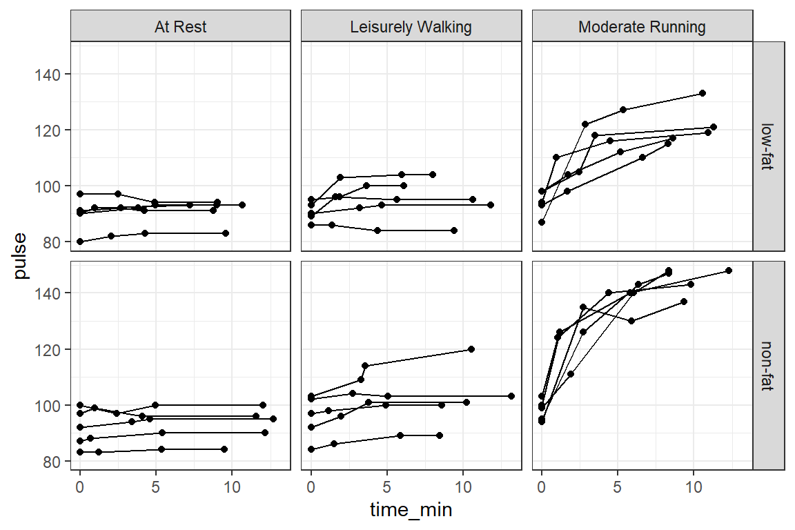
14.2.3.2 Loess - Moving Average Smoothers
df_ex_long %>%
  ggplot(aes(x = time_min,
             y = pulse,
             color = diet)) +
  geom_line(aes(group = id)) +
  facet_grid(~ exertype) +
  theme_bw() +
  geom_smooth(method = "loess",
              se = FALSE,
              size = 2,
              span = 5) +
  theme(legend.position = c(0.08, 0.85),
        legend.background = element_rect(color = "black")) +
  labs(title = "Raw Pulse Trajectories",
       subtitle = "By Exercise and Diet Groupings",
       x = "Time (Minutes Post-Baseline)",
       y = "Pulse (Beats per Minute)",
       color = "Diet Plan")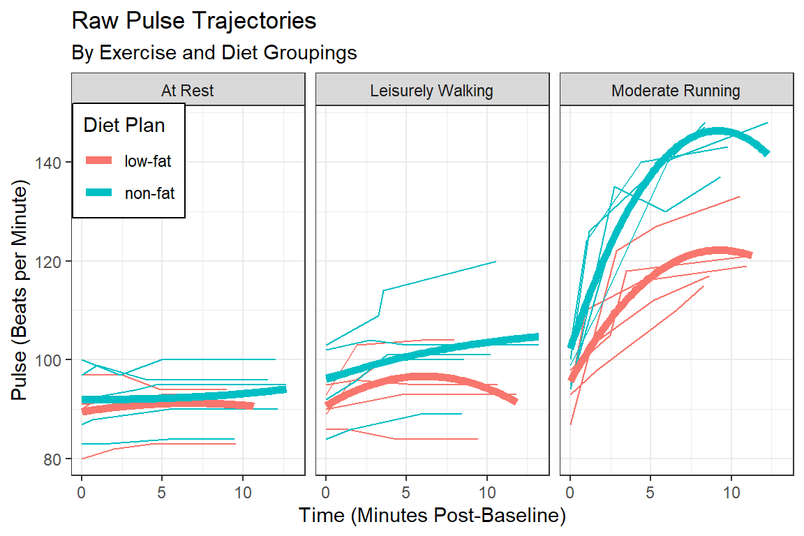
14.3 Multilevel Modeling
14.3.1 Null Model
Est | (SE) | p | |
|---|---|---|---|
(Intercept) | 102.13 | (2.54) | < .001*** |
id.var__(Intercept) | 165.84 | ||
Residual.var__Observation | 109.39 | ||
Note. Est = estimated regresssion coefficient for fixed effects and varaince/covariance estimates for random effects. p = significance from Wald t-test for parameter estimate using Satterthwaite's method for degrees of freedom. | |||
* p < .05. ** p < .01. *** p < .001. | |||
14.3.2 ICC & R-squared
# Intraclass Correlation Coefficient

    Adjusted ICC: 0.603
Unadjusted ICC: 0.603# R2 for Mixed Models
Conditional R2: 0.603
Marginal R2: 0.00014.3.3 Add fixed effects: level specific
14.3.3.1 Fit nested models
# Null Model (random intercept only)
fit_lmer_0ml <- lmerTest::lmer(pulse ~ 1 + (1 | id),
                               data = df_ex_long,
                               REML = FALSE)

# Add quadratic time
fit_lmer_1ml <- lmerTest::lmer(pulse ~ time_min + I(time_min^2) + (1 | id),
                               data = df_ex_long,
                               REML = FALSE)

# Add main effects for 2 interventions (person-specific, i.e. level-2 factors)
fit_lmer_2ml <- lmerTest::lmer(pulse ~ diet + exertype + time_min + I(time_min^2) + (1 | id),
                               data = df_ex_long,
                               REML = FALSE)

# Add interaction between level-2 factors
fit_lmer_3ml <- lmerTest::lmer(pulse ~ diet*exertype + time_min + I(time_min^2) + (1 | id),
                               data = df_ex_long,
                               REML = FALSE)

# Add exercise interacting with [time & time-squared]
fit_lmer_4ml <- lmerTest::lmer(pulse ~ diet*exertype + exertype*time_min + exertype*I(time_min^2) + (1 | id),
                               data = df_ex_long,
                               REML = FALSE)

# Add diet interacting with [time & time-squared]
fit_lmer_5ml <- lmerTest::lmer(pulse ~ diet*exertype*time_min + diet*exertype*I(time_min^2) + (1 | id),
                               data = df_ex_long,
REML = FALSE)apaSupp::tab_lmers(list("M0" = fit_lmer_0re,
"M1" = fit_lmer_1ml,
"M2" = fit_lmer_2ml),
narrow = TRUE)
| M0 | M1 | M2 | |||
|---|---|---|---|---|---|---|
Variable | b | (SE) | b | (SE) | b | (SE) |
(Intercept) | 102.13 | (2.54) *** | 94.05 | (2.71) *** | 79.30 | (2.46) *** |
time_min | 3.57 | (0.65) *** | 3.58 | (0.64) *** | ||
I(time_min^2) | -0.21 | (0.06) *** | -0.21 | (0.06) *** | ||
diet | ||||||
low-fat | — | — | ||||
non-fat | 8.36 | (2.21) *** | ||||
exertype | ||||||
At Rest | — | — | ||||
Leisurely Walking | 5.20 | (2.70) | ||||
Moderate Running | 26.43 | (2.70) *** | ||||
id.var__(Intercept) | 165.84 | 167.58 | 19.46 | |||
Residual.var__Observation | 109.39 | 67.47 | 67.47 | |||
AIC | 964 | 928 | 885 | |||
BIC | 972 | 942 | 907 | |||
Log-likelihood | -479 | -459 | -434 | |||
Note. | ||||||
* p < .05. ** p < .01. *** p < .001. | ||||||
apaSupp::tab_lmers(list("M3" = fit_lmer_3ml,
                        "M4" = fit_lmer_4ml,
                        "M5" = fit_lmer_5ml),
                   narrow = TRUE)
| M3 | M4 | M5 | |||
|---|---|---|---|---|---|---|
Variable | b | (SE) | b | (SE) | b | (SE) |
(Intercept) | 82.15 | (2.64) *** | 89.89 | (2.69) *** | 89.81 | (2.78) *** |
diet | ||||||
low-fat | — | — | — | — | — | — |
non-fat | 2.89 | (3.36) | 1.99 | (3.45) | 2.11 | (3.89) |
exertype | ||||||
At Rest | — | — | — | — | — | — |
Leisurely Walking | 3.81 | (3.34) | 0.84 | (3.78) | 1.40 | (3.92) |
Moderate Running | 19.71 | (3.34) *** | 0.53 | (3.77) | 5.71 | (3.92) |
time_min | 3.44 | (0.64) *** | 0.24 | (0.62) | 0.37 | (0.87) |
I(time_min^2) | -0.20 | (0.06) *** | -0.01 | (0.05) | -0.03 | (0.09) |
diet * exertype | ||||||
non-fat * Leisurely Walking | 2.83 | (4.73) | 3.70 | (4.86) | 2.53 | (5.50) |
non-fat * Moderate Running | 13.47 | (4.74) ** | 14.02 | (4.86) ** | 3.99 | (5.50) |
exertype * time_min | ||||||
Leisurely Walking * time_min | 1.17 | (0.87) | 1.09 | (1.17) | ||
Moderate Running * time_min | 8.19 | (0.90) *** | 5.77 | (1.20) *** | ||
exertype * I(time_min^2) | ||||||
Leisurely Walking * I(time_min^2) | -0.07 | (0.08) | -0.08 | (0.11) | ||
Moderate Running * I(time_min^2) | -0.48 | (0.08) *** | -0.33 | (0.11) ** | ||
diet * time_min | ||||||
non-fat * time_min | -0.17 | (1.14) | ||||
diet * I(time_min^2) | ||||||
non-fat * I(time_min^2) | 0.02 | (0.10) | ||||
diet * exertype * time_min | ||||||
non-fat * Leisurely Walking * time_min | 0.21 | (1.56) | ||||
non-fat * Moderate Running * time_min | 4.42 | (1.61) ** | ||||
diet * exertype * I(time_min^2) | ||||||
non-fat * Leisurely Walking * I(time_min^2) | 0.01 | (0.14) | ||||
non-fat * Moderate Running * I(time_min^2) | -0.27 | (0.15) | ||||
id.var__(Intercept) | 11.03 | 24.13 | 25.64 | |||
Residual.var__Observation | 67.52 | 20.95 | 15.32 | |||
AIC | 881 | 785 | 769 | |||
BIC | 909 | 824 | 825 | |||
Log-likelihood | -431 | -379 | -365 | |||
Note. | ||||||
* p < .05. ** p < .01. *** p < .001. | ||||||
14.3.3.2 Evaluate Model Fit, i.e. variable significance
Data: df_ex_long
Models:
fit_lmer_1ml: pulse ~ time_min + I(time_min^2) + (1 | id)
fit_lmer_2ml: pulse ~ diet + exertype + time_min + I(time_min^2) + (1 | id)
fit_lmer_3ml: pulse ~ diet * exertype + time_min + I(time_min^2) + (1 | id)
fit_lmer_4ml: pulse ~ diet * exertype + exertype * time_min + exertype * I(time_min^2) + (1 | id)
fit_lmer_5ml: pulse ~ diet * exertype * time_min + diet * exertype * I(time_min^2) + (1 | id)
             npar    AIC    BIC  logLik -2*log(L)   Chisq Df Pr(>Chisq)
fit_lmer_1ml    5 927.70 941.64 -458.85    917.70
fit_lmer_2ml    8 884.96 907.26 -434.48    868.96  48.742  3  1.480e-10 ***
fit_lmer_3ml   10 881.11 908.99 -430.56    861.11   7.847  2    0.01977 *
fit_lmer_4ml   14 785.34 824.36 -378.67    757.34 103.776  4  < 2.2e-16 ***
fit_lmer_5ml   20 769.23 824.98 -364.62    729.23  28.108  6  8.968e-05 ***
---
Signif. codes: 0 '***' 0.001 '**' 0.01 '*' 0.05 '.' 0.1 ' ' 1apaSupp::tab_lmer_fits(list("M1" = fit_lmer_1ml,
"M2" = fit_lmer_2ml,
"M3" = fit_lmer_3ml,
"M4" = fit_lmer_4ml,
"M5" = fit_lmer_5ml))Model | AIC | BIC | RMSE |
| |
|---|---|---|---|---|---|
Conditional | Marginal | ||||
M1 | 927.70 | 941.64 | 7.22 | .748 | .121 |
M2 | 884.96 | 907.26 | 7.64 | .750 | .678 |
M3 | 881.11 | 908.99 | 7.80 | .750 | .710 |
M4 | 785.34 | 824.36 | 4.08 | .923 | .835 |
M5 | 769.23 | 824.98 | 3.46 | .944 | .850 |
Note. Larger values indicated better performance. Smaller values indicated better performance for Akaike's Information Criteria (AIC), Bayesian information criteria (BIC), and Root Mean Squared Error (RMSE). | |||||
14.3.4 Final Model
Refit via REML
fit_lmer_5re <- lmerTest::lmer(pulse ~ diet*exertype*time_min +
diet*exertype*I(time_min^2) + (1 | id),
data = df_ex_long,
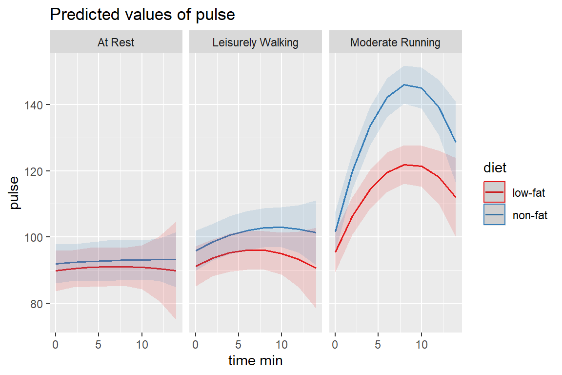
REML = TRUE)14.3.4.1 Visualize
interactions::interact_plot(fit_lmer_5re,
                            pred = time_min,
                            modx = diet,
                            mod2 = exertype,
                            interval = TRUE)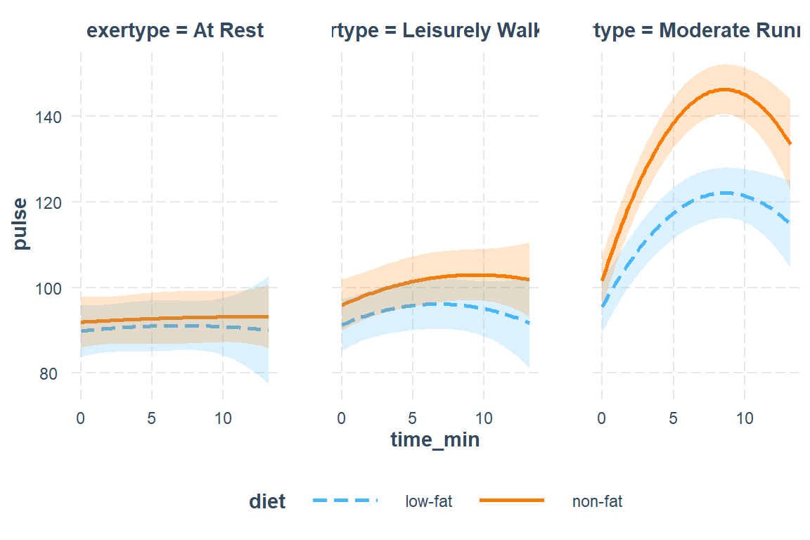
effects::Effect(focal.predictors = c("diet", "exertype", "time_min"),
                mod = fit_lmer_5re) %>%
  data.frame %>%
  ggplot(aes(x = time_min,
             y = fit,
             fill = diet,
             color = diet)) +
  geom_line(size = 1.5) +
  theme_bw() +
  facet_grid(~ exertype) +
  theme(legend.position = c(0.08, 0.85),
        legend.background = element_rect(color = "black")) +
  labs(title = "Raw Pulse Trajectories",
       subtitle = "By Exercise and Diet Groupings",
       x = "Time (Minutes Post-Baseline)",
       y = "Estimated Marginal Mean\nPulse (Beats per Minute)",
       fill = "Diet Plan",
       color = "Diet Plan")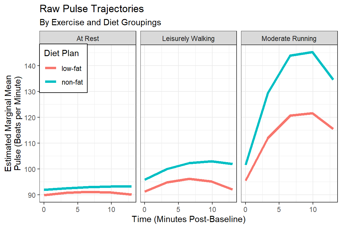
effects::Effect(focal.predictors = c("diet", "exertype", "time_min"),
                mod = fit_lmer_5re,
                xlevels = list("time_min" = seq(from = 0,
                                                to   = 12,
                                                by   = 0.5))) %>%
  data.frame %>%
  dplyr::mutate(diet = fct_rev(diet)) %>%  # reverse the order of the levels
  ggplot(aes(x = time_min,
             y = fit)) +
  geom_ribbon(aes(ymin = fit - se,
                  ymax = fit + se,
                  fill = diet),
              alpha = 0.3) +
  geom_line(aes(linetype = diet),
            size = 1) +
  theme_bw() +
  facet_grid(~ exertype) +
  theme(legend.position = c(0.12, 0.85),
        legend.background = element_rect(color = "black"),
        legend.key.width = unit(2, "cm")) +
  labs(title = "Raw Pulse Trajectories",
       subtitle = "By Randomized Exercise and Diet Intervention",
       x = "Time (Minutes Post-Baseline)",
       y = "Estimated Marginal Mean\nPulse (Beats per Minute)",
       fill = "Diet Plan",
       color = "Diet Plan",
       linetype = "Diet Plan") +
  scale_fill_manual(values = c("black", "gray50")) +
  scale_linetype_manual(values = c("solid", "longdash")) +
  scale_x_continuous(breaks = seq(from = 0, to = 14, by = 5))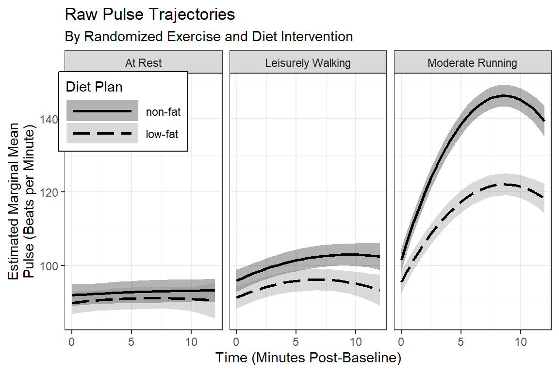
fit_lmer_5re %>%
  emmeans::emmeans(~ diet*exertype*time_min,
                   at = list("time_min" = seq(from = 0,
                                                to   = 12,
                                                by   = 0.5))) %>%
  data.frame %>%
  dplyr::mutate(diet = fct_rev(diet)) %>%  # reverse the order of the levels
  ggplot(aes(x = time_min,
             y = emmean)) +
  geom_ribbon(aes(ymin = emmean - SE,
                  ymax = emmean + SE,
                  fill = diet),
              alpha = 0.3) +
  geom_line(aes(linetype = diet),
            size = 1) +
  theme_bw() +
  facet_grid(~ exertype) +
  theme(legend.position = c(0.12, 0.85),
        legend.background = element_rect(color = "black"),
        legend.key.width = unit(2, "cm")) +
  labs(title = "Raw Pulse Trajectories",
       subtitle = "By Randomized Exercise and Diet Intervention",
       x = "Time (Minutes Post-Baseline)",
       y = "Estimated Marginal Mean\nPulse (Beats per Minute)",
       fill = "Diet Plan",
       color = "Diet Plan",
       linetype = "Diet Plan") +
  scale_fill_manual(values = c("black", "gray50")) +
  scale_linetype_manual(values = c("solid", "longdash")) +
  scale_x_continuous(breaks = seq(from = 0, to = 14, by = 5))
14.3.4.2 Pairwise Differences in Means
fit_lmer_5re %>%
  emmeans::emmeans(~diet|exertype*time_min,
                   at = list(time_min = c(0, 5, 10))) %>%
  pairs(adjust = "none") %>%
  data.frame() %>%
  dplyr::mutate(p_Unadj = apaSupp::p_num(p.value)) %>%
  dplyr::mutate(p_Adj = apaSupp::p_num(p.adjust(p.value, method = "fdr"))) %>%
  dplyr::mutate(SMD = estimate/apaSupp::lmer_sd(fit_lmer_5re)) %>%
  dplyr::arrange(exertype, time_min) %>%
  dplyr::select("Exercise" = exertype,
                "Time, min" = time_min,
                "EMM Difference_Est" = estimate,
                "EMM Difference_(SE)" = SE,
                SMD,
                p_Unadj,
                p_Adj) %>%
  flextable::as_grouped_data(groups = "Exercise") %>%
  flextable::flextable() %>%
  flextable::separate_header() %>%
  apaSupp::theme_apa(caption = "Diet Differences in Estimated Marginal Mean Pulse for each Exercise Program",
                     general_note = "EMM = estimated marginal means. SMD = standardized mean difference. P-values given both unadjusted (Unadj) and adjusted (Adj) via the method of Benjamini, Hochberg, and Yekutieli to control the false discovery rate (FDR)") %>%
flextable::hline(part = "header", i = 1)Exercise | Time, min | EMM Difference | SMD | p | ||
|---|---|---|---|---|---|---|
Est | (SE) | Unadj | Adj | |||
At Rest | ||||||
0.00 | -2.10 | 4.32 | -0.30 | .629 | .687 | |
5.00 | -1.73 | 4.26 | -0.24 | .687 | .687 | |
10.00 | -2.28 | 4.49 | -0.32 | .613 | .687 | |
Leisurely Walking | ||||||
0.00 | -4.63 | 4.32 | -0.65 | .290 | .436 | |
5.00 | -5.58 | 4.17 | -0.79 | .190 | .342 | |
10.00 | -7.89 | 4.43 | -1.11 | .083 | .248 | |
Moderate Running | ||||||
0.00 | -6.09 | 4.32 | -0.86 | .167 | .342 | |
5.00 | -21.11 | 4.23 | -2.98 | < .001*** | < .001*** | |
10.00 | -23.63 | 4.42 | -3.34 | < .001*** | < .001*** | |
Note. EMM = estimated marginal means. SMD = standardized mean difference. P-values given both unadjusted (Unadj) and adjusted (Adj) via the method of Benjamini, Hochberg, and Yekutieli to control the false discovery rate (FDR) | ||||||