13 MLM, Longitudinal: Hox ch 5 - student GPA

install.packages("devtools")
devtools::install_github("sarbearschwartz/apaSupp") # updated 9/17/2025

Load/activate these packages

library(haven)     
library(tidyverse)    
library(flextable)
library(apaSupp)      # Not on CRAN, on GitHub (see above)
library(psych)
library(VIM)         
library(naniar) 
library(lme4)        
library(lmerTest)
library(optimx)
library(performance)
library(interactions)
library(effects)
library(emmeans)
library(ggResidpanel)
library(HLMdiag)
library(sjPlot)
library(sjstats)

13.1 Background

The text “Multilevel Analysis: Techniques and Applications, Third Edition” (Hox, Moerbeek, and Van de Schoot 2017) has a companion website which includes links to all the data files used throughout the book (housed on the book’s GitHub repository).

The following example is used through out Hox, Moerbeek, and Van de Schoot (2017)’s chapater 5.

The GPA for 200 college students were followed for 6 consecutive semesters (simulated). Job status was also measured as number of hours worked for the same size occations. Time-invariant covariates are the student’s gender and high school GPA. The variable admitted will not be used.

df_raw <- haven::read_sav("data/gpa2long.sav") %>% 
  haven::as_factor() %>%             # retain the labels from SPSS --> factor
  haven::zap_label()

tibble::glimpse(df_raw)

Rows: 1,200
Columns: 7
$ student  <dbl> 1, 1, 1, 1, 1, 1, 2, 2, 2, 2, 2, 2, 3, 3, 3, 3, 3, 3, 4, 4, 4…
$ occas    <fct> year 1 semester 1, year 1 semester 2, year 2 semester 1, year…
$ gpa      <dbl> 2.3, 2.1, 3.0, 3.0, 3.0, 3.3, 2.2, 2.5, 2.6, 2.6, 3.0, 2.8, 2…
$ job      <fct> 2 hours, 2 hours, 2 hours, 2 hours, 2 hours, 2 hours, 2 hours…
$ sex      <fct> female, female, female, female, female, female, male, male, m…
$ highgpa  <dbl> 2.8, 2.8, 2.8, 2.8, 2.8, 2.8, 2.5, 2.5, 2.5, 2.5, 2.5, 2.5, 2…
$ admitted <fct> yes, yes, yes, yes, yes, yes, no, no, no, no, no, no, yes, ye…

df_raw %>% 
  dplyr::select(occas, job) %>% 
  table(useNA = "always")

                   job
occas               no job 1 hour 2 hours 3 hours 4 or more hours <NA>
  year 1 semester 1      0      0     172      28               0    0
  year 1 semester 2      0      0     169      31               0    0
  year 2 semester 1      0      7     159      34               0    0
  year 2 semester 2      0      5     169      26               0    0
  year 3 semester 1      0     18     150      32               0    0
  year 3 semester 2      0     22     148      30               0    0
  <NA>                   0      0       0       0               0    0

df_gpa_long <- df_raw %>% 
  dplyr::mutate(student = factor(student)) %>% 
  dplyr::mutate(sem = case_when(occas == "year 1 semester 1" ~ 1,
                                occas == "year 1 semester 2" ~ 2,
                                occas == "year 2 semester 1" ~ 3,
                                occas == "year 2 semester 2" ~ 4,
                                occas == "year 3 semester 1" ~ 5,
                                occas == "year 3 semester 2" ~ 6)) %>% 
  dplyr::mutate(job = fct_drop(job)) %>% 
  dplyr::mutate(hrs = case_when(job == "no job" ~ 0,
                                job == "1 hour" ~ 1,
                                job == "2 hours" ~ 2,
                                job == "3 hours" ~ 3,
                                job == "4 or more hours" ~ 4)) %>%  
  dplyr::select(student, sex, highgpa, sem, job, hrs, gpa) %>% 
  dplyr::arrange(student, sem)

tibble::glimpse(df_gpa_long)

Rows: 1,200
Columns: 7
$ student <fct> 1, 1, 1, 1, 1, 1, 2, 2, 2, 2, 2, 2, 3, 3, 3, 3, 3, 3, 4, 4, 4,…
$ sex     <fct> female, female, female, female, female, female, male, male, ma…
$ highgpa <dbl> 2.8, 2.8, 2.8, 2.8, 2.8, 2.8, 2.5, 2.5, 2.5, 2.5, 2.5, 2.5, 2.…
$ sem     <dbl> 1, 2, 3, 4, 5, 6, 1, 2, 3, 4, 5, 6, 1, 2, 3, 4, 5, 6, 1, 2, 3,…
$ job     <fct> 2 hours, 2 hours, 2 hours, 2 hours, 2 hours, 2 hours, 2 hours,…
$ hrs     <dbl> 2, 2, 2, 2, 2, 2, 2, 3, 2, 2, 2, 2, 2, 2, 2, 3, 2, 2, 3, 2, 2,…
$ gpa     <dbl> 2.3, 2.1, 3.0, 3.0, 3.0, 3.3, 2.2, 2.5, 2.6, 2.6, 3.0, 2.8, 2.…

df_gpa_long %>% 
  psych::headTail(top = 10) %>% 
  flextable::flextable() %>% 
  apaSupp::theme_apa(caption = "Data in Long Format")

**Table 13.1**
Data in Long Format
student	sex	highgpa	sem	job	hrs	gpa
1	female	2.8	1	2 hours	2	2.3
1	female	2.8	2	2 hours	2	2.1
1	female	2.8	3	2 hours	2	3
1	female	2.8	4	2 hours	2	3
1	female	2.8	5	2 hours	2	3
1	female	2.8	6	2 hours	2	3.3
2	male	2.5	1	2 hours	2	2.2
2	male	2.5	2	3 hours	3	2.5
2	male	2.5	3	2 hours	2	2.6
2	male	2.5	4	2 hours	2	2.6
		...	...		...	...
200	male	3.4	3	2 hours	2	3.4
200	male	3.4	4	2 hours	2	3.5
200	male	3.4	5	1 hour	1	3.3
200	male	3.4	6	1 hour	1	3.4

df_gpa_wide <- df_gpa_long %>% 
  tidyr::pivot_wider(names_from = sem,
                     values_from = c(job, hrs, gpa),
                     names_sep = "_")

tibble::glimpse(df_gpa_wide)

Rows: 200
Columns: 21
$ student <fct> 1, 2, 3, 4, 5, 6, 7, 8, 9, 10, 11, 12, 13, 14, 15, 16, 17, 18,…
$ sex     <fct> female, male, female, male, male, female, male, female, male, …
$ highgpa <dbl> 2.8, 2.5, 2.5, 3.8, 3.1, 2.9, 2.3, 3.9, 2.0, 2.8, 3.9, 2.9, 3.…
$ job_1   <fct> 2 hours, 2 hours, 2 hours, 3 hours, 2 hours, 2 hours, 3 hours,…
$ job_2   <fct> 2 hours, 3 hours, 2 hours, 2 hours, 2 hours, 3 hours, 2 hours,…
$ job_3   <fct> 2 hours, 2 hours, 2 hours, 2 hours, 2 hours, 3 hours, 3 hours,…
$ job_4   <fct> 2 hours, 2 hours, 3 hours, 2 hours, 2 hours, 2 hours, 2 hours,…
$ job_5   <fct> 2 hours, 2 hours, 2 hours, 2 hours, 2 hours, 3 hours, 2 hours,…
$ job_6   <fct> 2 hours, 2 hours, 2 hours, 2 hours, 2 hours, 3 hours, 2 hours,…
$ hrs_1   <dbl> 2, 2, 2, 3, 2, 2, 3, 2, 2, 2, 2, 3, 2, 2, 2, 2, 2, 3, 2, 2, 2,…
$ hrs_2   <dbl> 2, 3, 2, 2, 2, 3, 2, 2, 2, 2, 3, 2, 2, 2, 2, 2, 2, 2, 2, 2, 2,…
$ hrs_3   <dbl> 2, 2, 2, 2, 2, 3, 3, 2, 3, 2, 2, 2, 2, 2, 3, 2, 2, 2, 2, 2, 2,…
$ hrs_4   <dbl> 2, 2, 3, 2, 2, 2, 2, 2, 2, 3, 2, 2, 2, 2, 3, 2, 3, 2, 3, 2, 2,…
$ hrs_5   <dbl> 2, 2, 2, 2, 2, 3, 2, 2, 2, 2, 2, 2, 2, 2, 3, 2, 3, 2, 2, 2, 2,…
$ hrs_6   <dbl> 2, 2, 2, 2, 2, 3, 2, 2, 2, 2, 2, 2, 2, 2, 2, 2, 2, 3, 3, 2, 2,…
$ gpa_1   <dbl> 2.3, 2.2, 2.4, 2.5, 2.8, 2.5, 2.4, 2.8, 2.8, 2.8, 2.6, 2.6, 2.…
$ gpa_2   <dbl> 2.1, 2.5, 2.9, 2.7, 2.8, 2.4, 2.4, 2.8, 2.7, 2.8, 2.9, 3.0, 3.…
$ gpa_3   <dbl> 3.0, 2.6, 3.0, 2.4, 2.8, 2.4, 2.8, 3.1, 2.7, 3.0, 3.2, 2.3, 3.…
$ gpa_4   <dbl> 3.0, 2.6, 2.8, 2.7, 3.0, 2.3, 2.6, 3.3, 3.1, 2.7, 3.6, 2.9, 3.…
$ gpa_5   <dbl> 3.0, 3.0, 3.3, 2.9, 2.9, 2.7, 3.0, 3.3, 3.1, 3.0, 3.6, 3.1, 3.…
$ gpa_6   <dbl> 3.3, 2.8, 3.4, 2.7, 3.1, 2.8, 3.0, 3.4, 3.5, 3.0, 3.8, 3.3, 3.…

df_gpa_wide %>% 
  dplyr::select(sex,
                "High School GPA" = highgpa, 
                "Initial College GPA" = gpa_1, 
                "Initial Job" = job_1, 
                "Initial Hrs" = hrs_1) %>% 
  apaSupp::tab1(split = "sex",
                caption = "Demographic Summary by Sex")

**Table 13.2**
Demographic Summary by Sex
	Total N = 200	male n = 95 (47.5%)	female n = 105 (52.5%)	p-value
High School GPA	2.99 (0.60)	3.03 (0.59)	2.95 (0.60)	.309
Initial College GPA	2.59 (0.31)	2.55 (0.31)	2.63 (0.31)	.095
Initial Job				.192
1 hour	0 (0.0%)	0 (0.0%)	0 (0.0%)
2 hours	172 (86.0%)	78 (82.1%)	94 (89.5%)
3 hours	28 (14.0%)	17 (17.9%)	11 (10.5%)
Initial Hrs				.192
2	172 (86.0%)	78 (82.1%)	94 (89.5%)
3	28 (14.0%)	17 (17.9%)	11 (10.5%)
Note. Continuous variables are summarized with means (SD) and significant group differences assessed via independent t-tests. Categorical variables are summarized with counts (%) and significant group differences assessed via Chi-squared tests for independence.
* p < .05. p < .01. * p < .001.

df_gpa_wide %>% 
  dplyr::select(sex, gpa_1, gpa_2, gpa_3, gpa_4, gpa_5, gpa_6) %>% 
  apaSupp::tab1(split = "sex",
                caption = "Hox Table 5.2 (page 77) GPA means at six occations, for male and female students")

**Table 13.3**
Hox Table 5.2 (page 77) GPA means at six occations, for male and female students
	Total N = 200	male n = 95 (47.5%)	female n = 105 (52.5%)	p-value
gpa_1	2.59 (0.31)	2.55 (0.31)	2.63 (0.31)	.095
gpa_2	2.72 (0.34)	2.67 (0.32)	2.76 (0.35)	.048*
gpa_3	2.81 (0.35)	2.74 (0.36)	2.87 (0.34)	.010**
gpa_4	2.92 (0.36)	2.82 (0.35)	3.01 (0.34)	< .001***
gpa_5	3.02 (0.36)	2.91 (0.36)	3.11 (0.33)	< .001***
gpa_6	3.13 (0.38)	3.03 (0.38)	3.23 (0.35)	< .001***
Note. Continuous variables are summarized with means (SD) and significant group differences assessed via independent t-tests. Categorical variables are summarized with counts (%) and significant group differences assessed via Chi-squared tests for independence.
* p < .05. p < .01. * p < .001.

13.2 MLM

13.2.1 Null Models and ICC

fit_lmer_0_re <- lmerTest::lmer(gpa ~ 1 + (1|student),
                                data = df_gpa_long,
                                REML = TRUE)

performance::icc(fit_lmer_0_re)

# Intraclass Correlation Coefficient

    Adjusted ICC: 0.369
  Unadjusted ICC: 0.369

Over a third of the variance in the 6 GPA measures is variance between individuals, and about two-thirds is variance within individuals across time, $\rho = .369$.

fit_lmer_1_re <- lmerTest::lmer(gpa ~ I(sem - 1) + (1|student),
                                data = df_gpa_long,
                                REML = TRUE)

performance::icc(fit_lmer_1_re)

# Intraclass Correlation Coefficient

    Adjusted ICC: 0.523
  Unadjusted ICC: 0.412

After accounting for the linear change in GPA over semesters, about half of the remaining variance in GPA scores is attributable to person-to-person difference.

Another way to say it, is about half of the variance in initial GPAs is due to student-to-student differences.

apaSupp::tab_lmers(list("M0: Null w/o Time" = fit_lmer_0_re,
                        "M1: Null w/Time"   = fit_lmer_1_re),
                   caption = "Null Models")

**Table 13.4**
Null Models
	M0: Null w/o Time			M1: Null w/Time
Variable	b	(SE)	p	b	(SE)	p
(Intercept)	2.87	(0.02)	< .001***	2.60	(0.02)	< .001***
I(sem - 1)				0.11	(0.00)	< .001***
student.var__(Intercept)	0.06			0.06
Residual.var__Observation	0.10			0.06
AIC	926			417
BIC	941			437
Log-likelihood	-460			-204
Note.
* p < .05. p < .01. * p < .001.

13.2.2 Fixed Effects

fit_lmer_0_ml <- lmerTest::lmer(gpa ~ 1 + (1|student),
                                data = df_gpa_long,
                                REML = FALSE)

fit_lmer_1_ml <- lmerTest::lmer(gpa ~ I(sem - 1) + (1|student),
                                data = df_gpa_long,
                                REML = FALSE)


fit_lmer_2_ml <- lmerTest::lmer(gpa ~ I(sem - 1) + hrs + (1|student),
                                data = df_gpa_long,
                                REML = FALSE)


fit_lmer_3_ml <- lmerTest::lmer(gpa ~ I(sem - 1) + hrs + highgpa + sex + (1|student),
                                data = df_gpa_long,
                                REML = FALSE)

apaSupp::tab_lmers(list("M2: Occ" = fit_lmer_1_ml, 
                        "M3: Job" = fit_lmer_2_ml, 
                        "M4: GPA, Sex" = fit_lmer_3_ml),
                   var_labels = c("(Intercept)" = "(Intercept)",
                                  "I(sem - 1)" = "Semester",
                                  "hrs" = "Hours Working",
                                  "highgpa" = "High School GPA",
                                  "sex" = "Sex",
                                  "male" = "Male",
                                  "female" = "Female"),
                   narrow = TRUE,
                   caption = "Hox Table 5.3 (page 78) Results of Multilevel Anlaysis of GPA, Fixed Effects",
                   general_note = "Intercept refers to population mean for a Male who is not working during their first semester")

**Table 13.5**
Hox Table 5.3 (page 78) Results of Multilevel Anlaysis of GPA, Fixed Effects
	M2: Occ		M3: Job		M4: GPA, Sex
Variable	b	(SE)	b	(SE)	b	(SE)
(Intercept)	2.60	(0.02) ***	2.97	(0.04) ***	2.64	(0.10) ***
Semester	0.11	(0.00) ***	0.10	(0.00) ***	0.10	(0.00) ***
Hours Working			-0.17	(0.02) ***	-0.17	(0.02) ***
High School GPA					0.08	(0.03) **
Sex
Male					—	—
Female					0.15	(0.03) ***
student.var__(Intercept)	0.06		0.05		0.04
Residual.var__Observation	0.06		0.06		0.06
AIC	402		318		297
BIC	422		344		332
Log-likelihood	-197		-154		-141
Note. Intercept refers to population mean for a Male who is not working during their first semester
* p < .05. p < .01. * p < .001.

tab_lmer_fits(list("M0: Null w/o Time" = fit_lmer_0_re,
                   "M1: Null w/Time"   = fit_lmer_1_re, 
                   "M2: Occ"           = fit_lmer_1_ml, 
                   "M3: Job"           = fit_lmer_2_ml, 
                   "M4: GPA, Sex"      = fit_lmer_3_ml))

**Table 13.6**
Comparison of MLM Performane Metrics
Model	AIC	BIC	RMSE	$R^2$
Model	AIC	BIC	RMSE	Conditional	Marginal
M0: Null w/o Time	919.46	934.73	0.29	.369	< .001
M1: Null w/Time	401.65	422.01	0.22	.625	.213
M2: Occ	401.65	422.01	0.22	.624	.214
M3: Job	318.40	343.85	0.22	.622	.263
M4: GPA, Sex	296.76	332.39	0.22	.625	.319
Note. Larger $R^2$ values indicated better performance. Smaller values indicated better performance for Akaike's Information Criteria (AIC), Bayesian information criteria (BIC), and Root Mean Squared Error (RMSE).

anova(fit_lmer_0_ml, fit_lmer_1_ml, fit_lmer_2_ml, fit_lmer_3_ml)

Data: df_gpa_long
Models:
fit_lmer_0_ml: gpa ~ 1 + (1 | student)
fit_lmer_1_ml: gpa ~ I(sem - 1) + (1 | student)
fit_lmer_2_ml: gpa ~ I(sem - 1) + hrs + (1 | student)
fit_lmer_3_ml: gpa ~ I(sem - 1) + hrs + highgpa + sex + (1 | student)
              npar    AIC    BIC  logLik -2*log(L)   Chisq Df Pr(>Chisq)    
fit_lmer_0_ml    3 919.46 934.73 -456.73    913.46                          
fit_lmer_1_ml    4 401.65 422.01 -196.82    393.65 519.807  1  < 2.2e-16 ***
fit_lmer_2_ml    5 318.40 343.85 -154.20    308.40  85.250  1  < 2.2e-16 ***
fit_lmer_3_ml    7 296.76 332.39 -141.38    282.76  25.639  2  2.707e-06 ***
---
Signif. codes:  0 '***' 0.001 '**' 0.01 '*' 0.05 '.' 0.1 ' ' 1

13.2.3 Variance Explained by linear TIME at Level ONE

lme4::VarCorr(fit_lmer_0_ml)  # baseline

 Groups   Name        Std.Dev.
 student  (Intercept) 0.23826 
 Residual             0.31239

lme4::VarCorr(fit_lmer_1_ml)  # model to compare

 Groups   Name        Std.Dev.
 student  (Intercept) 0.25172 
 Residual             0.24090

lme4::VarCorr(fit_lmer_0_ml) %>%  # baseline
  print(comp = c("Variance", "Std.Dev"),
        digits = 3)

 Groups   Name        Variance Std.Dev.
 student  (Intercept) 0.0568   0.238   
 Residual             0.0976   0.312

lme4::VarCorr(fit_lmer_1_ml) %>%  # model to compare
  print(comp = c("Variance", "Std.Dev"),
        digits = 3)

 Groups   Name        Variance Std.Dev.
 student  (Intercept) 0.0634   0.252   
 Residual             0.0580   0.241

performance::r2(fit_lmer_1_ml)

# R2 for Mixed Models

  Conditional R2: 0.624
     Marginal R2: 0.214

performance::r2(fit_lmer_1_ml, by_group = TRUE)

# Explained Variance by Level

Level   |     R2
----------------
Level 1 |  0.405
student | -0.116

13.2.3.1 Raudenbush and Bryk

Explained variance is a proportion of first-level variance only
A good option when the multilevel sampling process is is close to two-stage simple random sampling

Raudenbush and Bryk Approximate Formula - Level 1 approximate \[ approx \;R^2_1 = \frac{\sigma^2_{e-BL} - \sigma^2_{e-MC}} {\sigma^2_{e-BL} } \tag{Hox 4.8} \]

(0.098 - 0.058) / 0.098

[1] 0.4081633

13.2.3.2 Snijders and Bosker

Snijders and Bosker Formula - Level 1

Random Intercepts Models Only, address potential negative $R^2$ issue \[ R^2_1 = 1 - \frac{\sigma^2_{e-MC} + \sigma^2_{u0-MC}} {\sigma^2_{e-BL} + \sigma^2_{u0-BL}} \]

1 - (0.058 + 0.063)/(0.098 + 0.057)

[1] 0.2193548

13.2.4 Variance Explained by linear TIME at Level TWO

13.2.4.1 Raudenbush and Bryk

Raudenbush and Bryk Approximate Formula - Level 2 \[ approx \; R^2_s = \frac{\sigma^2_{u0-BL} - \sigma^2_{u0-MC}} {\sigma^2_{u0-BL} } \tag{Hox 4.9} \]

(0.057 - 0.063)/ 0.057

[1] -0.1052632

YIKES! Negative Variance explained!

13.2.4.2 Snijders and Bosker

Snijders and Bosker Formula Extended - Level 2 \[ R^2_2 = 1 - \frac{\frac{\sigma^2_{e-MC}}{B} + \sigma^2_{u0-MC}} {\frac{\sigma^2_{e-BL}}{B} + \sigma^2_{u0-BL}} \]

$B$ is the average size of the Level 2 units. Technically, you should use the harmonic mean, but unless the clusters differ greatly in size, it doesn’t make a huge difference.

1 - (0.058/6 + 0.063) / (0.098/6 + 0.057)

[1] 0.009090909

Reason: The intercept only model overestimates the variance at the occasion level and underestimates the variance at the subject level (see chapter 4 of Hox, Moerbeek, and Van de Schoot (2017))

13.2.5 Random Effects

fit_lmer_3_re <- lmerTest::lmer(gpa ~ I(sem-1) + hrs + highgpa + sex + 
                                  (1|student),
                                data = df_gpa_long,
                                REML = TRUE)


fit_lmer_4_re <- lmerTest::lmer(gpa ~ I(sem-1) + hrs + highgpa + sex +
                                  (I(sem-1)|student),
                                data = df_gpa_long,
                                REML = TRUE,
                                control = lmerControl(optimizer ="Nelder_Mead"))

anova(fit_lmer_3_re, fit_lmer_4_re, refit = FALSE)

Data: df_gpa_long
Models:
fit_lmer_3_re: gpa ~ I(sem - 1) + hrs + highgpa + sex + (1 | student)
fit_lmer_4_re: gpa ~ I(sem - 1) + hrs + highgpa + sex + (I(sem - 1) | student)
              npar    AIC    BIC  logLik -2*log(L) Chisq Df Pr(>Chisq)    
fit_lmer_3_re    7 328.84 364.47 -157.42    314.84                        
fit_lmer_4_re    9 219.93 265.75 -100.97    201.94 112.9  2  < 2.2e-16 ***
---
Signif. codes:  0 '***' 0.001 '**' 0.01 '*' 0.05 '.' 0.1 ' ' 1

13.2.6 Cross-Level Interaction

fit_lmer_4_ml <- lmerTest::lmer(gpa ~ I(sem-1) + 
                                  hrs + highgpa + sex + 
                                  (I(sem-1)|student),
                                data = df_gpa_long,
                                REML = FALSE)

fit_lmer_5_ml <- lmerTest::lmer(gpa ~ I(sem-1) + 
                                  hrs + highgpa + sex + 
                                  I(sem-1):sex + 
                                  (I(sem-1)|student),
                                data = df_gpa_long,
                                REML = FALSE)

fit_lmer_5_re <- lmerTest::lmer(gpa ~ I(sem-1) + 
                                  hrs + highgpa + sex + 
                                  I(sem-1):sex + 
                                  (I(sem-1)|student),
                                data = df_gpa_long,
                                REML = TRUE)

apaSupp::tab_lmers(list("M5: Occ Rand"   = fit_lmer_4_ml,
                        "M6: Xlevel Int" = fit_lmer_5_ml),
                   var_labels = c("(Intercept)" = "(Intercept)",
                                  "I(sem - 1)" = "Semester",
                                  "hrs" = "Hours Working",
                                  "sexfemale" = "Sex: Female vs. Male",
                                  "highgpa" = "High School GPA",
                                  "I(sem - 1):sexfemale" = "Semester X Sex"),
                   caption = "Hox Table 5.4 (page 80) Results of Multilevel Anlaysis of GPA, Varying Effects for Occation",
                   general_note = "Intercept refers to population mean for a Male who is not working during their first semester and had a high school GPA = 0.",
                   d = 3)

**Table 13.7**
Hox Table 5.4 (page 80) Results of Multilevel Anlaysis of GPA, Varying Effects for Occation
	M5: Occ Rand			M6: Xlevel Int
Variable	b	(SE)	p	b	(SE)	p
(Intercept)	2.558	(0.092)	< .0010***	2.581	(0.092)	< .0010***
Semester	0.103	(0.006)	< .0010***	0.088	(0.008)	< .0010***
Hours Working	-0.131	(0.017)	< .0010***	-0.132	(0.017)	< .0010***
High School GPA	0.089	(0.026)	< .0010***	0.089	(0.026)	< .0010***
sex
male	—	—		—	—
female	0.116	(0.031)	< .0010***	0.076	(0.035)	.0305*
I(sem - 1) * sex
I(sem - 1) * female				0.030	(0.011)	.0076**
student.var__(Intercept)	0.038			0.038
student.cov__(Intercept).I(sem - 1)	-0.002			-0.002
student.var__I(sem - 1)	0.004			0.004
Residual.var__Observation	0.042			0.042
AIC	188			183
BIC	234			234
Log-likelihood	-85.1			-81.5
Note. Intercept refers to population mean for a Male who is not working during their first semester and had a high school GPA = 0.
* p < .05. p < .01. * p < .001.

anova(fit_lmer_4_ml, fit_lmer_5_ml)

Data: df_gpa_long
Models:
fit_lmer_4_ml: gpa ~ I(sem - 1) + hrs + highgpa + sex + (I(sem - 1) | student)
fit_lmer_5_ml: gpa ~ I(sem - 1) + hrs + highgpa + sex + I(sem - 1):sex + (I(sem - 1) | student)
              npar    AIC    BIC  logLik -2*log(L)  Chisq Df Pr(>Chisq)   
fit_lmer_4_ml    9 188.12 233.93 -85.059    170.12                        
fit_lmer_5_ml   10 182.97 233.87 -81.486    162.97 7.1464  1   0.007511 **
---
Signif. codes:  0 '***' 0.001 '**' 0.01 '*' 0.05 '.' 0.1 ' ' 1

13.2.7 Visualize the Model

apaSupp::tab_lmer(fit_lmer_5_re,
                  d = 3)

**Table 13.8**
Parameter Estimates for Mixed Effects Regression
	Est	(SE)	p
(Intercept)	2.580	(0.093)	< .0010***
I(sem - 1)	0.088	(0.008)	< .0010***
hrs	-0.132	(0.017)	< .0010***
highgpa	0.089	(0.026)	< .0010***
sex
male	—	—
female	0.076	(0.035)	.0317*
I(sem - 1) * sex
I(sem - 1) * female	0.030	(0.011)	.0079**
student.var__(Intercept)	0.039
student.cov__(Intercept).I(sem - 1)	-0.002
student.var__I(sem - 1)	0.004
Residual.var__Observation	0.042
Note. Est = estimated regresssion coefficient for fixed effects and varaince/covariance estimates for random effects. p = significance from Wald t-test for parameter estimate using Satterthwaite's method for degrees of freedom.
* p < .05. p < .01. * p < .001.

13.2.7.1 Using `interactions::interact_plot()`

interactions::interact_plot(model = fit_lmer_5_re,
                            pred = sem,
                            modx = sex,
                            interval = TRUE)

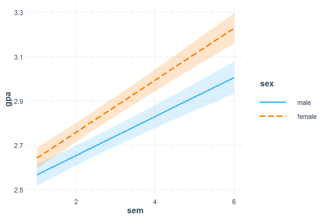
Figure 13.1
Hox Figure 5.4 (page 82) Multilevel model (M6) comapring linear increase in GPA over semester, but student’s sex.

interactions::interact_plot(model = fit_lmer_5_re,
                            pred = sem,
                            modx = sex,
                            mod2 = hrs,
                            mod2.values = c(1, 2, 3),
                            interval = TRUE)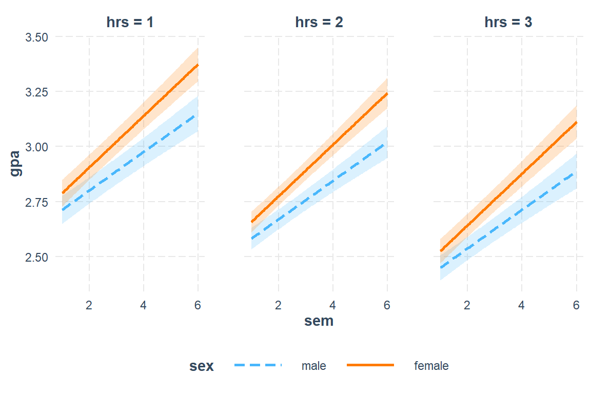

interactions::interact_plot(model = fit_lmer_5_re,
                            pred = sem,
                            modx = sex,
                            mod2 = highgpa,
                            mod2.values = c(2, 3, 4),
                            interval = TRUE)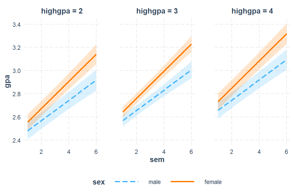

13.2.7.2 Using `emmeans::emmeans()` & `ggplot`

fit_lmer_5_re %>% 
  emmeans::emmeans(~sem*sex,
                   at = list(sem = 1:6))

 sem sex    emmean     SE  df lower.CL upper.CL
   1 male     2.57 0.0253 198     2.52     2.62
   2 male     2.65 0.0230 198     2.61     2.70
   3 male     2.74 0.0234 197     2.70     2.79
   4 male     2.83 0.0263 197     2.78     2.88
   5 male     2.92 0.0311 197     2.86     2.98
   6 male     3.01 0.0370 198     2.93     3.08
   1 female   2.64 0.0240 197     2.60     2.69
   2 female   2.76 0.0219 197     2.72     2.80
   3 female   2.88 0.0222 197     2.83     2.92
   4 female   2.99 0.0250 197     2.95     3.04
   5 female   3.11 0.0296 198     3.05     3.17
   6 female   3.23 0.0352 198     3.16     3.30

Degrees-of-freedom method: kenward-roger 
Confidence level used: 0.95

fit_lmer_5_re %>% 
  emmeans::emmeans(~sem*sex,
                   at = list(sem = 1:6)) %>% 
  data.frame() %>% 
  dplyr::mutate(sex = sex %>% 
                  forcats::fct_recode("Male" = "male",
                                      "Female" = "female") %>% 
                  forcats::fct_rev()) %>% 
  ggplot(aes(x = sem,
             y = emmean,
             group = sex)) +
  geom_ribbon(aes(ymin = emmean - SE,
                  ymax = emmean + SE,
                  fill = sex),
              alpha = .2) +
  geom_point(aes(shape = sex,
                 color = sex),
             size = 3) +
  geom_line(aes(linetype = sex,
                color = sex)) +
  theme_bw() +
  labs(x = "Semester",
       y = "Estimated Marginal Mean\nCollege GPA",
       fill = NULL,
       color = NULL,
       shape = NULL,
       linetype = NULL) +
  scale_x_continuous(breaks = 1:6) +
  scale_y_continuous(breaks = seq(from = 0, to = 4, by = .2)) +
  scale_linetype_manual(values = c("solid", "longdash")) +
  theme(legend.position = "inside",
        legend.position.inside = c(0, 1),
        legend.justification = c(-.1, 1.1),
        legend.key.width = unit(1.5, "cm"),
        legend.background = element_rect(color = "black"))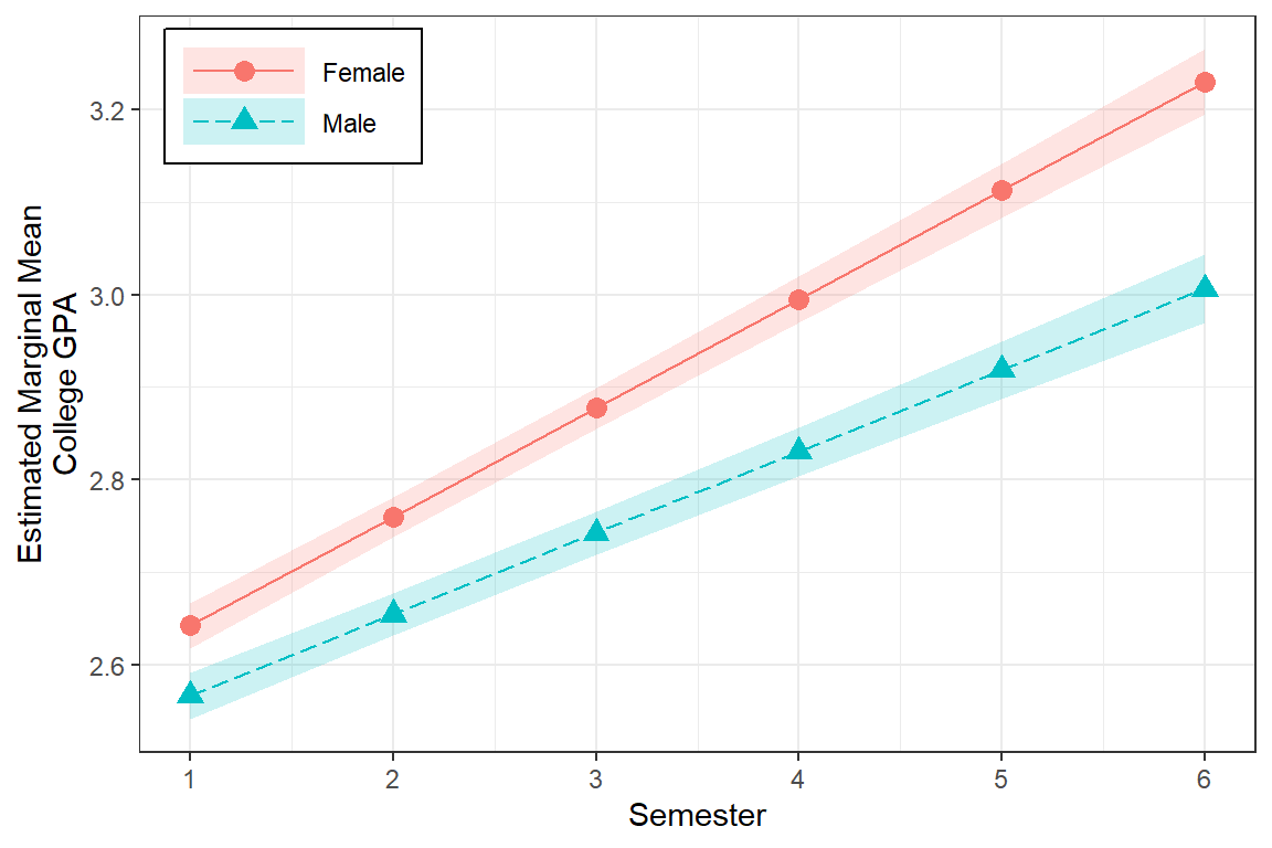

13.2.8 Effect Sizes

13.2.8.1 Standardized Parameters

effectsize::standardize_parameters(fit_lmer_5_re)

# Standardization method: refit

Parameter              | Std. Coef. |         95% CI
----------------------------------------------------
(Intercept)            |       0.18 | [ 0.02,  0.34]
sem - 1                |       0.38 | [ 0.31,  0.45]
hrs                    |      -0.14 | [-0.18, -0.11]
highgpa                |       0.13 | [ 0.06,  0.21]
sex [female]           |       0.51 | [ 0.29,  0.73]
sem - 1 × sex [female] |       0.13 | [ 0.03,  0.22]

13.2.8.2 R-squared type measures

performance::r2(fit_lmer_5_re)

# R2 for Mixed Models

  Conditional R2: 0.719
     Marginal R2: 0.306

performance::r2(fit_lmer_5_re, by_group = TRUE)

# Explained Variance by Level

Level   |    R2
---------------
Level 1 | 0.019
student | 0.336

13.2.8.3 Pairwise Differences in Means

fit_lmer_5_re %>% 
  emmeans::emmeans(~sex | sem,
                   at = list(sem = 1:6))

sem = 1:
 sex    emmean     SE  df lower.CL upper.CL
 male     2.57 0.0253 198     2.52     2.62
 female   2.64 0.0240 197     2.60     2.69

sem = 2:
 sex    emmean     SE  df lower.CL upper.CL
 male     2.65 0.0230 198     2.61     2.70
 female   2.76 0.0219 197     2.72     2.80

sem = 3:
 sex    emmean     SE  df lower.CL upper.CL
 male     2.74 0.0234 197     2.70     2.79
 female   2.88 0.0222 197     2.83     2.92

sem = 4:
 sex    emmean     SE  df lower.CL upper.CL
 male     2.83 0.0263 197     2.78     2.88
 female   2.99 0.0250 197     2.95     3.04

sem = 5:
 sex    emmean     SE  df lower.CL upper.CL
 male     2.92 0.0311 197     2.86     2.98
 female   3.11 0.0296 198     3.05     3.17

sem = 6:
 sex    emmean     SE  df lower.CL upper.CL
 male     3.01 0.0370 198     2.93     3.08
 female   3.23 0.0352 198     3.16     3.30

Degrees-of-freedom method: kenward-roger 
Confidence level used: 0.95

fit_lmer_5_re %>% 
  emmeans::emmeans(~sex | sem,
                   at = list(sem = 1:6)) %>% 
  pairs()

sem = 1:
 contrast      estimate     SE  df t.ratio p.value
 male - female  -0.0755 0.0349 198  -2.164  0.0317

sem = 2:
 contrast      estimate     SE  df t.ratio p.value
 male - female  -0.1051 0.0318 197  -3.307  0.0011

sem = 3:
 contrast      estimate     SE  df t.ratio p.value
 male - female  -0.1347 0.0323 197  -4.167  <.0001

sem = 4:
 contrast      estimate     SE  df t.ratio p.value
 male - female  -0.1642 0.0364 198  -4.517  <.0001

sem = 5:
 contrast      estimate     SE  df t.ratio p.value
 male - female  -0.1938 0.0429 198  -4.515  <.0001

sem = 6:
 contrast      estimate     SE  df t.ratio p.value
 male - female  -0.2233 0.0510 198  -4.376  <.0001

Degrees-of-freedom method: kenward-roger

fit_lmer_5_re %>% 
  emmeans::emmeans(~sex | sem,
                   at = list(sem = 1:6)) %>% 
  pairs(adjust = "none") %>% 
  data.frame() %>% 
  dplyr::mutate(p_Unadj = apaSupp::p_num(p.value)) %>% 
  dplyr::mutate(p_Adj = apaSupp::p_num(p.adjust(p.value, method = "fdr"))) %>% 
  dplyr::mutate(SMD = estimate/apaSupp::lmer_sd(fit_lmer_5_re)) %>% 
  dplyr::select("Semester" = sem,
                "EMM Difference_Est" = estimate, 
                "EMM Difference_(SE)" = SE,
                SMD,
                p_Unadj,
                p_Adj) %>% 
    flextable::flextable() %>% 
  flextable::separate_header() %>% 
  apaSupp::theme_apa(caption = "Sex Differences in Estimated Marginal Mean Collegate GPA for each Semester",
                     general_note = "EMM = estimated marginal means. SMD = standardized mean difference. P-values given both unadjusted (Unadj) and adjusted (Adj) via the method of Benjamini, Hochberg, and Yekutieli to control the false discovery rate (FDR)") %>% 
  flextable::hline(part = "header", i = 1)

**Table 13.9**
Sex Differences in Estimated Marginal Mean Collegate GPA for each Semester
Semester	EMM Difference		SMD	p
Semester	Est	(SE)	SMD	Unadj	Adj
1	-0.08	0.03	-0.26	.032*	.032*
2	-0.11	0.03	-0.37	.001**	.001**
3	-0.13	0.03	-0.47	< .001***	< .001***
4	-0.16	0.04	-0.57	< .001***	< .001***
5	-0.19	0.04	-0.68	< .001***	< .001***
6	-0.22	0.05	-0.78	< .001***	< .001***
Note. EMM = estimated marginal means. SMD = standardized mean difference. P-values given both unadjusted (Unadj) and adjusted (Adj) via the method of Benjamini, Hochberg, and Yekutieli to control the false discovery rate (FDR)

13.2.8.4 Simple Slopes

fit_lmer_5_re %>% 
  emmeans::emtrends( ~ sex, var = "sem")

 sex    sem.trend     SE  df lower.CL upper.CL
 male      0.0878 0.0080 199   0.0721    0.104
 female    0.1174 0.0076 199   0.1024    0.132

Degrees-of-freedom method: kenward-roger 
Confidence level used: 0.95

13.2.9 Significance

13.2.9.1 Fixed Effects

The Likelyhood Ratio Test (Deviance Difference Test) is best for establishing significance of fixed effects.

Wald-tests

summary(fit_lmer_5_re)

Linear mixed model fit by REML. t-tests use Satterthwaite's method [
lmerModLmerTest]
Formula: gpa ~ I(sem - 1) + hrs + highgpa + sex + I(sem - 1):sex + (I(sem -  
    1) | student)
   Data: df_gpa_long

REML criterion at convergence: 202

Scaled residuals: 
    Min      1Q  Median      3Q     Max 
-3.0001 -0.5275 -0.0151  0.5261  3.3470 

Random effects:
 Groups   Name        Variance Std.Dev. Corr 
 student  (Intercept) 0.038669 0.19664       
          I(sem - 1)  0.003678 0.06065  -0.19
 Residual             0.041592 0.20394       
Number of obs: 1200, groups:  student, 200

Fixed effects:
                       Estimate Std. Error         df t value Pr(>|t|)    
(Intercept)           2.580e+00  9.300e-02  2.909e+02  27.742  < 2e-16 ***
I(sem - 1)            8.784e-02  7.995e-03  1.967e+02  10.987  < 2e-16 ***
hrs                  -1.317e-01  1.725e-02  1.038e+03  -7.632  5.2e-14 ***
highgpa               8.852e-02  2.648e-02  1.947e+02   3.343 0.000993 ***
sexfemale             7.553e-02  3.491e-02  1.976e+02   2.164 0.031668 *  
I(sem - 1):sexfemale  2.956e-02  1.102e-02  1.957e+02   2.683 0.007921 ** 
---
Signif. codes:  0 '***' 0.001 '**' 0.01 '*' 0.05 '.' 0.1 ' ' 1

Correlation of Fixed Effects:
            (Intr) I(s-1) hrs    highgp sexfml
I(sem - 1)  -0.139                            
hrs         -0.426  0.054                     
highgpa     -0.872  0.001  0.022              
sexfemale   -0.265  0.312  0.030  0.066       
I(sm-1):sxf  0.088 -0.724 -0.008  0.000 -0.429

F-test with Satterthwaite adjusted degrees of freedom

anova(fit_lmer_5_re)

Type III Analysis of Variance Table with Satterthwaite's method
                Sum Sq Mean Sq NumDF   DenDF  F value    Pr(>F)    
I(sem - 1)     14.3609 14.3609     1  197.45 345.2775 < 2.2e-16 ***
hrs             2.4229  2.4229     1 1037.87  58.2545 5.204e-14 ***
highgpa         0.4649  0.4649     1  194.68  11.1772 0.0009931 ***
sex             0.1948  0.1948     1  197.59   4.6827 0.0316679 *  
I(sem - 1):sex  0.2994  0.2994     1  195.74   7.1984 0.0079211 ** 
---
Signif. codes:  0 '***' 0.001 '**' 0.01 '*' 0.05 '.' 0.1 ' ' 1

13.2.9.2 Random Effects

Likelyhood Ratio Tests (Deviance Difference Test), by single term deletion

lmerTest::ranova(fit_lmer_5_re)

ANOVA-like table for random-effects: Single term deletions

Model:
gpa ~ I(sem - 1) + hrs + highgpa + sex + (I(sem - 1) | student) + I(sem - 1):sex
                                     npar  logLik    AIC    LRT Df Pr(>Chisq)
<none>                                 10 -101.01 222.01                     
I(sem - 1) in (I(sem - 1) | student)    8 -154.30 324.59 106.58  2  < 2.2e-16
                                        
<none>                                  
I(sem - 1) in (I(sem - 1) | student) ***
---
Signif. codes:  0 '***' 0.001 '**' 0.01 '*' 0.05 '.' 0.1 ' ' 1