16 GEE, Binary Outcome: Respiratory Illness

16.1 PREPARATION

16.1.1 Load Packages

install.packages("devtools")
devtools::install_github("sarbearschwartz/apaSupp") # updated 10/14/2025

Load/activate these packages

library(tidyverse)    
library(flextable)
library(apaSupp)      # Not on CRAN, on GitHub (see above)
library(psych) 
library(lme4)         
library(lmerTest)
library(corrplot)      
library(geepack)       
library(MuMIn)  
library(interactions)
library(performance)      

library(HSAUR)        # package with the dataset

16.1.2 Background

This dataset was used as an example in Chapter 11 of “A Handbook of Statistical Analysis using R” by Brian S. Everitt and Torsten Hothorn. The authors include this data set in their HSAUR package on CRAN.

The Background

In each of two centers, eligible patients were randomly assigned to active treatment or placebo. During the treatment, the respiratory status (categorized poor or good) was determined at each of four, monthly visits. The trial recruited 111 participants (54 in the active group, 57 in the placebo group) and there were no missing data for either the responses or the covariates.

The Research Question

The question of interest is to assess whether the treatment is effective and to estimate its effect.

Note: We are NOT interested in change over time, but rather mean differences in the treatment group compared to the placebo group, net of any potential confounding due to age, sex, and site.

The Data

Note that the data (555 observations on the following 7 variables) are in long form, i.e, repeated measurements are stored as additional rows in the data frame.

• Indicators

• subject the patient ID, a factor with levels 1 to 111

• centre the study center, a factor with levels 1 and 2
  

• month the month, each patient was examined at months 0, 1, 2, 3 and 4

• Outcome or dependent variable

• status the respiratory status (response variable), a factor with levels poor and good

• Main predictor or independent variable of interest

• treatment the treatment arm, a factor with levels placebo and treatment

• Time-invariant Covariates to control for

• sex a factor with levels female and male
  

• age the age of the patient

16.1.3 Read in the data

data("respiratory", package = "HSAUR")

str(respiratory)

'data.frame':   555 obs. of  7 variables:
 $ centre   : Factor w/ 2 levels "1","2": 1 1 1 1 1 1 1 1 1 1 ...
 $ treatment: Factor w/ 2 levels "placebo","treatment": 1 1 1 1 1 1 1 1 1 1 ...
 $ sex      : Factor w/ 2 levels "female","male": 1 1 1 1 1 1 1 1 1 1 ...
 $ age      : num  46 46 46 46 46 28 28 28 28 28 ...
 $ status   : Factor w/ 2 levels "poor","good": 1 1 1 1 1 1 1 1 1 1 ...
 $ month    : Ord.factor w/ 5 levels "0"<"1"<"2"<"3"<..: 1 2 3 4 5 1 2 3 4 5 ...
 $ subject  : Factor w/ 111 levels "1","2","3","4",..: 1 1 1 1 1 2 2 2 2 2 ...

tibble::glimpse(respiratory)

Rows: 555
Columns: 7
$ centre    <fct> 1, 1, 1, 1, 1, 1, 1, 1, 1, 1, 1, 1, 1, 1, 1, 1, 1, 1, 1, 1, …
$ treatment <fct> placebo, placebo, placebo, placebo, placebo, placebo, placeb…
$ sex       <fct> female, female, female, female, female, female, female, fema…
$ age       <dbl> 46, 46, 46, 46, 46, 28, 28, 28, 28, 28, 23, 23, 23, 23, 23, …
$ status    <fct> poor, poor, poor, poor, poor, poor, poor, poor, poor, poor, …
$ month     <ord> 0, 1, 2, 3, 4, 0, 1, 2, 3, 4, 0, 1, 2, 3, 4, 0, 1, 2, 3, 4, …
$ subject   <fct> 1, 1, 1, 1, 1, 2, 2, 2, 2, 2, 3, 3, 3, 3, 3, 4, 4, 4, 4, 4, …

16.1.4 Wide Format

Wide format has one line per participant.

df_resp_wide <- respiratory %>% 
  tidyr::spread(key = month,
                value = status,
                sep = "_") %>% 
  dplyr::rename("BL_status" = "month_0") %>% 
  dplyr::arrange(subject) %>% 
  dplyr::select(subject, centre, 
                sex, age, treatment, 
                BL_status, starts_with("month")) %>% 
  dplyr::mutate_if(is.factor, ~forcats::fct_relabel(.x, stringr::str_to_title))

tibble::glimpse(df_resp_wide)

Rows: 111
Columns: 10
$ subject   <fct> 1, 2, 3, 4, 5, 6, 7, 8, 9, 10, 11, 12, 13, 14, 15, 16, 17, 1…
$ centre    <fct> 1, 1, 1, 1, 1, 1, 1, 1, 1, 1, 1, 1, 1, 1, 1, 1, 1, 1, 1, 1, …
$ sex       <fct> Female, Female, Female, Female, Male, Female, Female, Female…
$ age       <dbl> 46, 28, 23, 44, 13, 34, 43, 28, 31, 37, 30, 14, 23, 30, 20, …
$ treatment <fct> Placebo, Placebo, Treatment, Placebo, Placebo, Treatment, Pl…
$ BL_status <fct> Poor, Poor, Good, Good, Good, Poor, Poor, Poor, Good, Good, …
$ month_1   <fct> Poor, Poor, Good, Good, Good, Poor, Good, Poor, Good, Poor, …
$ month_2   <fct> Poor, Poor, Good, Good, Good, Poor, Poor, Poor, Good, Good, …
$ month_3   <fct> Poor, Poor, Good, Good, Good, Poor, Good, Poor, Good, Good, …
$ month_4   <fct> Poor, Poor, Good, Poor, Good, Poor, Good, Poor, Good, Poor, …

df_resp_wide %>% 
  psych::headTail(top = 10, bottom = 10) %>% 
  flextable::flextable() %>% 
  apaSupp::theme_apa(caption = "Wide Format")

Table 16.1
Wide Format

subject	centre	sex	age	treatment	BL_status	month_1	month_2	month_3	month_4
1	1	Female	46	Placebo	Poor	Poor	Poor	Poor	Poor
2	1	Female	28	Placebo	Poor	Poor	Poor	Poor	Poor
3	1	Female	23	Treatment	Good	Good	Good	Good	Good
4	1	Female	44	Placebo	Good	Good	Good	Good	Poor
5	1	Male	13	Placebo	Good	Good	Good	Good	Good
6	1	Female	34	Treatment	Poor	Poor	Poor	Poor	Poor
7	1	Female	43	Placebo	Poor	Good	Poor	Good	Good
8	1	Female	28	Treatment	Poor	Poor	Poor	Poor	Poor
9	1	Female	31	Treatment	Good	Good	Good	Good	Good
10	1	Female	37	Placebo	Good	Poor	Good	Good	Poor
			...
102	2	Female	48	Placebo	Good	Good	Poor	Poor	Poor
103	2	Female	20	Treatment	Poor	Good	Good	Good	Good
104	2	Male	39	Placebo	Good	Poor	Good	Poor	Poor
105	2	Female	28	Treatment	Poor	Good	Poor	Poor	Poor
106	2	Male	38	Placebo	Poor	Poor	Poor	Poor	Poor
107	2	Female	43	Treatment	Good	Good	Good	Good	Good
108	2	Male	39	Treatment	Poor	Good	Good	Good	Good
109	2	Female	68	Treatment	Poor	Good	Good	Good	Good
110	2	Male	63	Treatment	Good	Good	Good	Good	Good
111	2	Female	31	Treatment	Good	Good	Good	Good	Good

16.1.5 Long Format

Long format has one line per observation.

df_resp_long <- df_resp_wide%>% 
  tidyr::gather(key = month,
                value = status,
                starts_with("month")) %>% 
  dplyr::mutate(month = str_sub(month, start = -1) %>% as.numeric) %>% 
  dplyr::mutate(status = case_when(status == "Poor" ~ 0,
                                   status == "Good" ~ 1)) %>% 
  dplyr::arrange(subject, month) %>% 
  dplyr::select(subject, centre, sex, age, treatment, BL_status, month, status)

tibble::glimpse(df_resp_long)

Rows: 444
Columns: 8
$ subject   <fct> 1, 1, 1, 1, 2, 2, 2, 2, 3, 3, 3, 3, 4, 4, 4, 4, 5, 5, 5, 5, …
$ centre    <fct> 1, 1, 1, 1, 1, 1, 1, 1, 1, 1, 1, 1, 1, 1, 1, 1, 1, 1, 1, 1, …
$ sex       <fct> Female, Female, Female, Female, Female, Female, Female, Fema…
$ age       <dbl> 46, 46, 46, 46, 28, 28, 28, 28, 23, 23, 23, 23, 44, 44, 44, …
$ treatment <fct> Placebo, Placebo, Placebo, Placebo, Placebo, Placebo, Placeb…
$ BL_status <fct> Poor, Poor, Poor, Poor, Poor, Poor, Poor, Poor, Good, Good, …
$ month     <dbl> 1, 2, 3, 4, 1, 2, 3, 4, 1, 2, 3, 4, 1, 2, 3, 4, 1, 2, 3, 4, …
$ status    <dbl> 0, 0, 0, 0, 0, 0, 0, 0, 1, 1, 1, 1, 1, 1, 1, 0, 1, 1, 1, 1, …

df_resp_long %>% 
  psych::headTail(top = 10, bottom = 10) %>% 
  flextable::flextable() %>% 
  apaSupp::theme_apa(caption = "Long Format")

Table 16.2
Long Format

subject	centre	sex	age	treatment	BL_status	month	status
1	1	Female	46	Placebo	Poor	1	0
1	1	Female	46	Placebo	Poor	2	0
1	1	Female	46	Placebo	Poor	3	0
1	1	Female	46	Placebo	Poor	4	0
2	1	Female	28	Placebo	Poor	1	0
2	1	Female	28	Placebo	Poor	2	0
2	1	Female	28	Placebo	Poor	3	0
2	1	Female	28	Placebo	Poor	4	0
3	1	Female	23	Treatment	Good	1	1
3	1	Female	23	Treatment	Good	2	1
			...			...	...
109	2	Female	68	Treatment	Poor	3	1
109	2	Female	68	Treatment	Poor	4	1
110	2	Male	63	Treatment	Good	1	1
110	2	Male	63	Treatment	Good	2	1
110	2	Male	63	Treatment	Good	3	1
110	2	Male	63	Treatment	Good	4	1
111	2	Female	31	Treatment	Good	1	1
111	2	Female	31	Treatment	Good	2	1
111	2	Female	31	Treatment	Good	3	1
111	2	Female	31	Treatment	Good	4	1

16.2 EXPLORATORY DATA ANLAYSIS

16.2.1 Summary Statistics

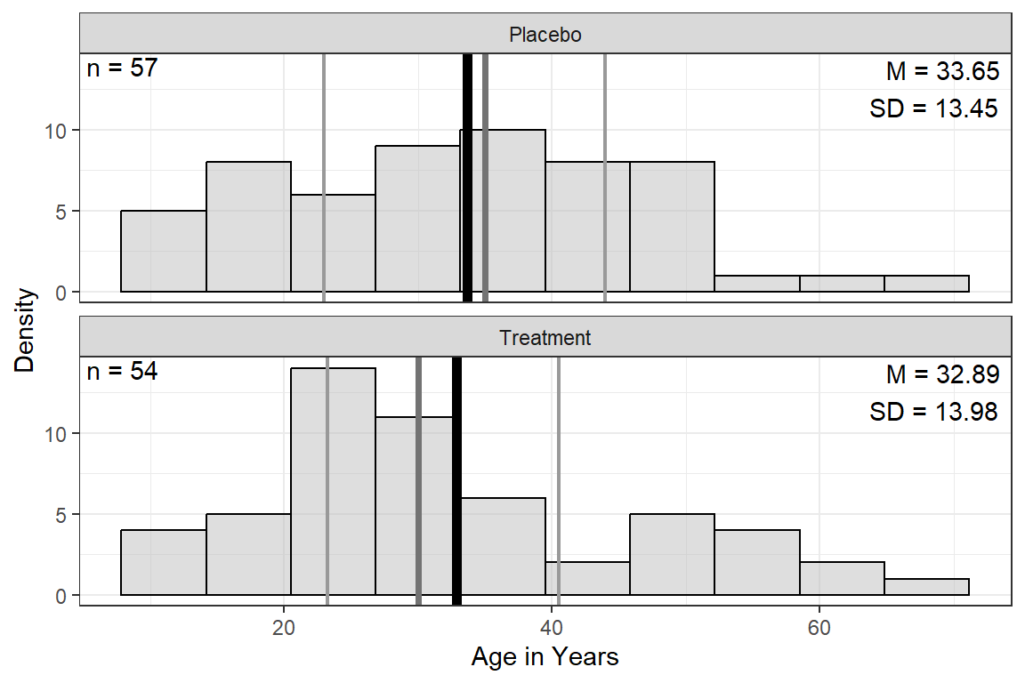
16.2.1.1 Demographics and Baseline Measure

Notice that numerical summaries are computed for all variables, even the categorical variables (i.e. factors). The have an * after the variable name to remind you that the mean, sd, and se are of limited use.

Notice: the mean age is 33

df_resp_wide %>% 
  apaSupp::tab_desc(caption = "Description of Participant Age")

Table 16.3
Description of Participant Age

	NA	M	SD	min	Q1	Mdn	Q3	max
age	0	33.28	13.65	11.00	23.00	31.00	43.00	68.00
Note. N = 111. NA = not available or missing; Mdn = median; Q1 = 25th percentile; Q3 = 75th percentile.

df_resp_wide %>%  
  dplyr::select(treatment,
                "Center" = centre, 
                "Sex" = sex, 
                "Age" = age, 
                "Baseline Status" = BL_status) %>% 
  apaSupp::tab1(split = "treatment",
                caption = "Participant Demographics",
                p_note = "apa1")

Table 16.4
Participant Demographics

	Total N = 111	Placebo n = 57 (51.4%)	Treatment n = 54 (48.6%)	p-value
Center				1.000
1	56 (50.5%)	29 (50.9%)	27 (50.0%)
2	55 (49.5%)	28 (49.1%)	27 (50.0%)
Sex				.028*
Female	88 (79.3%)	40 (70.2%)	48 (88.9%)
Male	23 (20.7%)	17 (29.8%)	6 (11.1%)
Age	33.28 (13.65)	33.65 (13.45)	32.89 (13.98)	.771
Baseline Status				1.000
Poor	61 (55.0%)	31 (54.4%)	30 (55.6%)
Good	50 (45.0%)	26 (45.6%)	24 (44.4%)
Note. Continuous variables are summarized with means (SD) and significant group differences assessed via independent t-tests. Categorical variables are summarized with counts (%) and significant group differences assessed via Chi-squared tests for independence.
* p < .05.

16.2.1.2 Status Over Time

df_resp_wide %>% 
  dplyr::select(treatment,
                "Month One" = month_1, 
                "Month Two" = month_2, 
                "Month Three" = month_3, 
                "Month Four" = month_4) %>% 
  apaSupp::tab1(split = "treatment",
                caption = "Respiratory Status Over Time",
                p_note = "apa2")

Table 16.5
Respiratory Status Over Time

	Total N = 111	Placebo n = 57 (51.4%)	Treatment n = 54 (48.6%)	p-value
Month One				.060
Poor	46 (41.4%)	29 (50.9%)	17 (31.5%)
Good	65 (58.6%)	28 (49.1%)	37 (68.5%)
Month Two				.002**
Poor	51 (45.9%)	35 (61.4%)	16 (29.6%)
Good	60 (54.1%)	22 (38.6%)	38 (70.4%)
Month Three				.008**
Poor	46 (41.4%)	31 (54.4%)	15 (27.8%)
Good	65 (58.6%)	26 (45.6%)	39 (72.2%)
Month Four				.068
Poor	52 (46.8%)	32 (56.1%)	20 (37.0%)
Good	59 (53.2%)	25 (43.9%)	34 (63.0%)
Note. . .
** p < .01.

Correlation between repeated observations:

df_resp_wide %>% 
  dplyr::select(starts_with("month")) %>% 
  dplyr::mutate_all(function(x) x == "Good") %>% 
  cor() %>% 
  corrplot::corrplot.mixed()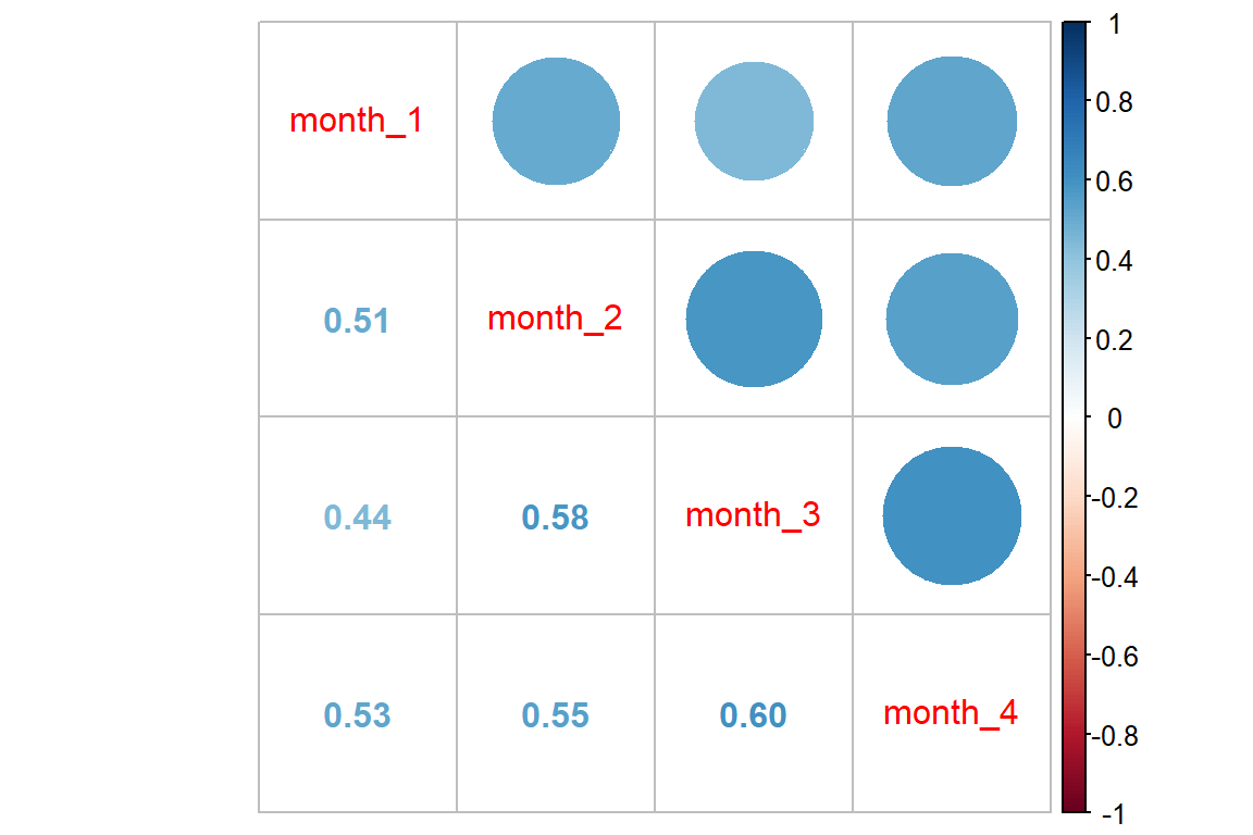

16.2.2 Visualization

16.2.2.1 Age

df_resp_wide %>% 
  apaSupp::spicy_histos(age,
                        split = treatment,
                        lab = "Age in Years")

16.2.2.2 Status by Age

df_resp_wide %>% 
  dplyr::mutate(n_good = furniture::rowsums(month_1 == "Good", 
                                            month_2 == "Good",
                                            month_3 == "Good",
                                            month_4 == "Good")) %>% 
  ggplot(aes(x = age,
             y = n_good)) +
  geom_count() +
  geom_smooth() +
  theme_bw() +
  labs(x = "Age in Years",
       y = "Number of Visits out of Four\nwith 'Good' Respiration")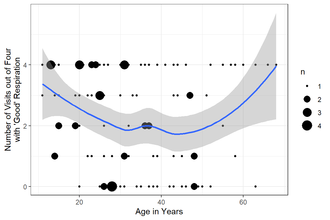

16.2.2.3 Status Over Time

It appears that status is fairly constant over time.

df_resp_long %>% 
  dplyr::group_by(treatment, month) %>% 
  dplyr::summarise(n = n(),
                   prop_good = mean(status),
                   prop_sd = sd(status),
                   prop_se = prop_sd/sqrt(n)) %>% 
  ggplot(aes(x = month,
             y = prop_good,
             group = treatment,
             color = treatment)) +
  geom_errorbar(aes(ymin = prop_good - prop_se,
                    ymax = prop_good + prop_se),
                width = .25,
                show.legend = FALSE) +
  geom_point(aes(shape = treatment),
             size = 2) +
  geom_line(aes(linetype = treatment)) +
  theme_bw() +
  labs(x = "Time, months",
       y = "Observed Proportion of Participants\nwith 'Good' Respiratory Status",
       color = NULL,
       shape = NULL,
       linetype = NULL) +
  scale_linetype_manual(values = c("solid", "longdash")) +
  theme(legend.position = "bottom",
        legend.key.width = unit(1.5, "cm"))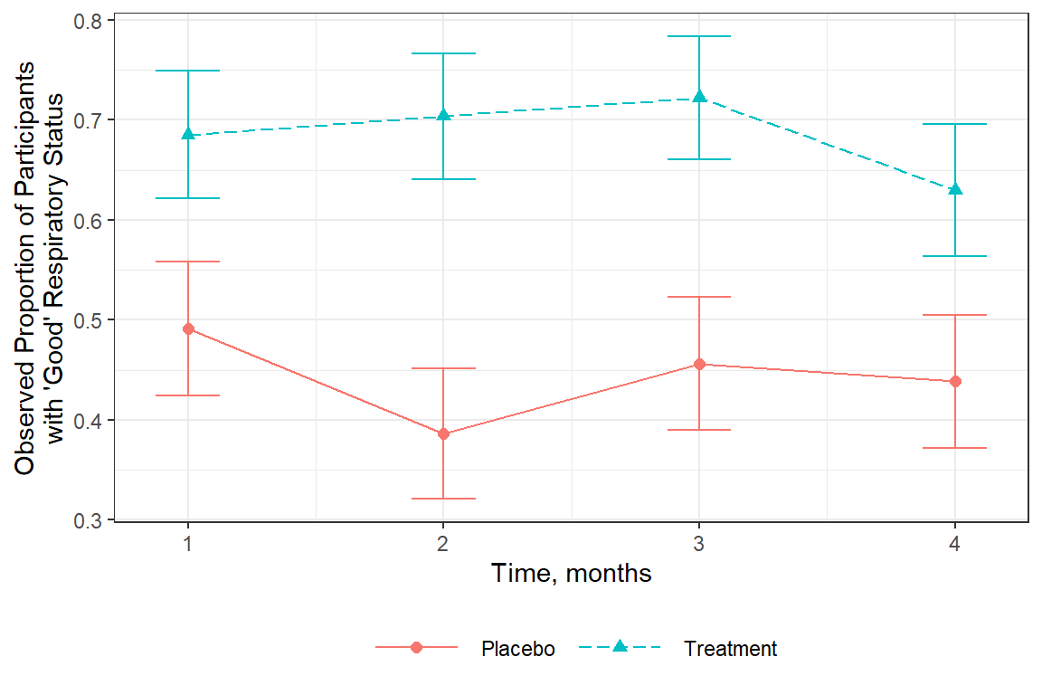

It is NOT the purpose of this analysis to investigate change over time!

Since status is largely stable over time, no linear (or even quadratic) effect of the month variable will be modeled.

Instead, the four observations on each subject are treated as correlated (at least with non-independent correlation structure in GEE), but no time trend will be included.

16.3 Generalized Estimating Equations (GEE)

Again, since participants age is likely to be a risk at either end of the spectrum, the potential quadratic effect of age will be modeled. Age is also being grand-mean centered to make the intercept more meaningful.

16.3.1 Indepdendence

Using an "independence" correlation structure is equivalent to using a GLM analysis (logistic regression in this case) and is never appropriate for repeated measures data. It is only being done here for comparison purposes.

fit_geeglm_in <- geepack::geeglm(status ~ centre + treatment + sex + BL_status + 
                                   I(age-33) + I((age-33)^2),
                                 data = df_resp_long,
                                 family = binomial(link = "logit"),
                                 id = subject,
                                 waves = month,
                                 corstr = "independence",
                                 scale.fix = TRUE)

summary(fit_geeglm_in)

Call:
geepack::geeglm(formula = status ~ centre + treatment + sex + 
    BL_status + I(age - 33) + I((age - 33)^2), family = binomial(link = "logit"), 
    data = df_resp_long, id = subject, waves = month, corstr = "independence", 
    scale.fix = TRUE)

 Coefficients:
                     Estimate    Std.err   Wald Pr(>|W|)    
(Intercept)        -1.9685725  0.4457014 19.508 1.00e-05 ***
centre2             0.5347938  0.3795760  1.985 0.158858    
treatmentTreatment  1.3561814  0.3777999 12.886 0.000331 ***
sexMale             0.4263433  0.4832337  0.778 0.377630    
BL_statusGood       1.9193401  0.3772812 25.881 3.63e-07 ***
I(age - 33)        -0.0368535  0.0150120  6.027 0.014091 *  
I((age - 33)^2)     0.0025169  0.0007592 10.989 0.000917 ***
---
Signif. codes:  0 '***' 0.001 '**' 0.01 '*' 0.05 '.' 0.1 ' ' 1

Correlation structure = independence 
Scale is fixed.

Number of clusters:   111  Maximum cluster size: 4 

The results for GEE fit with the independence correlation structure produces results that are nearly identical to the GLM model.

16.3.2 Exchangeable

fit_geeglm_ex <- geepack::geeglm(status ~ centre + treatment + sex + BL_status + 
                                   I(age-33) + I((age-33)^2),
                                 data = df_resp_long,
                                 family = binomial(link = "logit"),
                                 id = subject,
                                 waves = month,
                                 corstr = "exchangeable",
                                 scale.fix = TRUE)

summary(fit_geeglm_ex)

Call:
geepack::geeglm(formula = status ~ centre + treatment + sex + 
    BL_status + I(age - 33) + I((age - 33)^2), family = binomial(link = "logit"), 
    data = df_resp_long, id = subject, waves = month, corstr = "exchangeable", 
    scale.fix = TRUE)

 Coefficients:
                    Estimate   Std.err  Wald Pr(>|W|)    
(Intercept)        -1.968572  0.445701 19.51  1.0e-05 ***
centre2             0.534794  0.379576  1.99  0.15886    
treatmentTreatment  1.356181  0.377800 12.89  0.00033 ***
sexMale             0.426343  0.483234  0.78  0.37763    
BL_statusGood       1.919340  0.377281 25.88  3.6e-07 ***
I(age - 33)        -0.036854  0.015012  6.03  0.01409 *  
I((age - 33)^2)     0.002517  0.000759 10.99  0.00092 ***
---
Signif. codes:  0 '***' 0.001 '**' 0.01 '*' 0.05 '.' 0.1 ' ' 1

Correlation structure = exchangeable 
Scale is fixed.

  Link = identity 

Estimated Correlation Parameters:
      Estimate Std.err
alpha    0.312  0.0521
Number of clusters:   111  Maximum cluster size: 4 

16.3.3 Auto-Regressive

fit_geeglm_ar <- geepack::geeglm(status ~ centre + treatment + sex + BL_status + 
                                   I(age-33) + I((age-33)^2),
                                 data = df_resp_long,
                                 family = binomial(link = "logit"),
                                 id = subject,
                                 waves = month,
                                 corstr = "ar1",
                                 scale.fix = TRUE)

summary(fit_geeglm_ar)

Call:
geepack::geeglm(formula = status ~ centre + treatment + sex + 
    BL_status + I(age - 33) + I((age - 33)^2), family = binomial(link = "logit"), 
    data = df_resp_long, id = subject, waves = month, corstr = "ar1", 
    scale.fix = TRUE)

 Coefficients:
                    Estimate   Std.err  Wald Pr(>|W|)    
(Intercept)        -1.949751  0.451399 18.66  1.6e-05 ***
centre2             0.627506  0.375800  2.79  0.09496 .  
treatmentTreatment  1.286413  0.377526 11.61  0.00066 ***
sexMale             0.388172  0.485677  0.64  0.42415    
BL_statusGood       1.942647  0.374568 26.90  2.1e-07 ***
I(age - 33)        -0.033646  0.014935  5.08  0.02427 *  
I((age - 33)^2)     0.002306  0.000755  9.32  0.00227 ** 
---
Signif. codes:  0 '***' 0.001 '**' 0.01 '*' 0.05 '.' 0.1 ' ' 1

Correlation structure = ar1 
Scale is fixed.

  Link = identity 

Estimated Correlation Parameters:
      Estimate Std.err
alpha    0.428  0.0552
Number of clusters:   111  Maximum cluster size: 4 

16.3.4 Paramgeter Estimates Table

apaSupp::tab_gees(list("Independent" = fit_geeglm_in,
                       "Exchangable" = fit_geeglm_ex,
                       "Autoregress" = fit_geeglm_ar),
                  narrow = TRUE)

Table 16.6
Compare GEE Models

	Independent		Exchangable		Autoregress
	OR	95% CI	OR	95% CI	OR	95% CI
centre
1	—	—	—	—	—	—
2	1.71	[0.81, 3.59]	1.71	[0.81, 3.59]	1.87	[0.90, 3.91]
treatment
Placebo	—	—	—	—	—	—
Treatment	3.88	[1.85, 8.14]***	3.88	[1.85, 8.14]***	3.62	[1.73, 7.59]***
sex
Female	—	—	—	—	—	—
Male	1.53	[0.59, 3.95]	1.53	[0.59, 3.95]	1.47	[0.57, 3.82]
BL_status
Poor	—	—	—	—	—	—
Good	6.82	[3.25, 14.28]***	6.82	[3.25, 14.28]***	6.98	[3.35, 14.54]***
I(age - 33)	0.96	[0.94, 0.99]*	0.96	[0.94, 0.99]*	0.97	[0.94, 1.00]*
I((age - 33)^2)	1.00	[1.00, 1.00]***	1.00	[1.00, 1.00]***	1.00	[1.00, 1.00]**
Note.
* p < .05. ** p < .01. *** p < .001.

16.3.5 Compare Models

MuMIn::QIC(fit_geeglm_in, 
           fit_geeglm_ex, 
           fit_geeglm_ar, 
           typeR = FALSE)

              QIC
fit_geeglm_in 491
fit_geeglm_ex 491
fit_geeglm_ar 492

16.3.5.1 Manual Extraction

fit_geeglm_ex %>% coef() %>% exp()

       (Intercept)            centre2 treatmentTreatment            sexMale 
             0.140              1.707              3.881              1.532 
     BL_statusGood        I(age - 33)    I((age - 33)^2) 
             6.816              0.964              1.003 

trt_EST <- summary(fit_geeglm_ex)$coeff["treatmentTreatment", "Estimate"] 
trt_EST

[1] 1.36

exp(trt_EST)

[1] 3.88

Trt_SE <- summary(fit_geeglm_ex)$coeff["treatmentTreatment", "Std.err"] 
Trt_SE

[1] 0.378

trt_95ci <- trt_EST + c(-1, +1)*1.96*Trt_SE
trt_95ci

[1] 0.616 2.097

exp(trt_95ci)

[1] 1.85 8.14

16.3.6 Final Model

16.3.6.1 Estimates on both the logit and odds-ratio scales

apaSupp::tab_gee(fit_geeglm_ex,
                 caption = "GEE: Final Model (exchangable)")

Table 16.7
GEE: Final Model (exchangable)

	Odds Ratio			Logit Scale
	OR	95% CI		b	(SE)		p
centre
1	—	—		—	—
2	1.71	[0.81, 3.59]		0.53	(0.38)		.159
treatment
Placebo	—	—		—	—
Treatment	3.88	[1.85, 8.14]		1.36	(0.38)		< .001***
sex
Female	—	—		—	—
Male	1.53	[0.59, 3.95]		0.43	(0.48)		.378
BL_status
Poor	—	—		—	—
Good	6.82	[3.25, 14.28]		1.92	(0.38)		< .001***
I(age - 33)	0.96	[0.94, 0.99]		-0.04	(0.02)		.014*
I((age - 33)^2)	1.00	[1.00, 1.00]		0.00	(0.00)		< .001***
(Intercept)				-1.97	(0.45)		< .001***
Note. N = 444 observations on 111 participants. Correlation structure: exchangeable
* p < .05. ** p < .01. *** p < .001.

16.3.6.2 Interpretation

• centre: Controlling for baseline status, sex, age, and treatment, participants at the two centers did not significantly differ in respiratory status during the intervention

• sex: Controlling for baseline status, center, age, and treatment, a participant’s respiratory status did not differ between the two sexes.

• BL_status: Controlling for sex, center, age, and treatment, those with good baseline status had nearly 7 times higher odds of having a good respiratory status, compared to participants that starts out poor.

• age: Controlling for baseline status, sex, center, and treatment, the role of age was non-linear, such that the odds of a good respiratory status was lowest for patients age 40 and better for those that were either younger or older.

Most importantly:

• treatment: Controlling for baseline status, sex, age, and center, those on the treatment had 3.88 time higher odds of having a good respiratory status, compared to similar participants that were randomized to the placebo.

16.3.7 Predicted Probabilities

16.3.7.1 Make predictions

What is the change a 40 year old man in poor condition at center 1 change of being rated as being in “Good” respiratory condition?

fit_geeglm_ex %>% 
  emmeans::emmeans(pairwise ~ treatment,
                   at = list(centre = "1",
                             sex = "Male",
                             age = 40,
                             BL_status = "Poor"),
                   type = "response")

$emmeans
 treatment  prob     SE  df lower.CL upper.CL
 Placebo   0.158 0.0548 437   0.0767    0.296
 Treatment 0.421 0.1160 437   0.2211    0.650

Covariance estimate used: vbeta 
Confidence level used: 0.95 
Intervals are back-transformed from the logit scale 

$contrasts
 contrast            odds.ratio     SE  df null t.ratio p.value
 Placebo / Treatment      0.258 0.0973 437    1  -3.590  0.0004

Tests are performed on the log odds ratio scale 

A 40 year old man in poor condition at center 1 has a 15.8% change of being rated as being in “Good” respiratory condition if he was randomized to placebo.

A 40 year old man in poor condition at center 1 has a 42.1% change of being rated as being in “Good” respiratory condition if he was randomized to placebo.

The odds ratio for treatment is:

(.421/(1 -.421) )/( .158/(1 - .158))

[1] 3.87

16.3.8 Marginal Plot to Visualize the Model

16.3.8.1 Quickest Version

The interactions::interact_plot() function can only investigate 3 variables at once:

• pred the x-axis (must be continuous)
• modx different lines (may be categorical or continuous)
• mod2 side-by-side panels (may be categorical or continuous)

All other variables must be held constant.

interactions::interact_plot(model = fit_geeglm_ex,   # model name
                            pred = age,               # x-axis
                            modx = treatment,         # lines
                            mod2 = sex,               # panels
                            data = df_resp_long,
                            at = list(centre = "1",
                                      BL_status = "Good"),  # hold constant
                            type = "mean_subject") +
  theme_bw()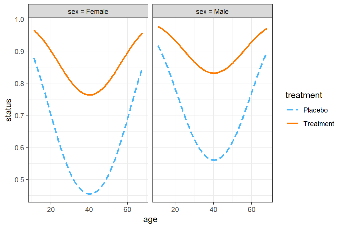

16.3.8.2 Full Version

Makes a dataset with all combinations

fit_geeglm_ex %>% 
  emmeans::emmeans(~ centre + treatment + sex + age + BL_status,
                   at = list(age = c(20, 35, 50)),
                   type = "response") %>% 
  data.frame()

   centre treatment    sex age BL_status  prob     SE  df lower.CL upper.CL
1       1   Placebo Female  20      Poor 0.257 0.0655 437   0.1494    0.404
2       2   Placebo Female  20      Poor 0.371 0.1211 437   0.1751    0.620
3       1 Treatment Female  20      Poor 0.572 0.0709 437   0.4310    0.703
4       2 Treatment Female  20      Poor 0.696 0.0901 437   0.4975    0.841
5       1   Placebo   Male  20      Poor 0.346 0.1033 437   0.1773    0.565
6       2   Placebo   Male  20      Poor 0.474 0.1190 437   0.2610    0.697
7       1 Treatment   Male  20      Poor 0.672 0.1335 437   0.3840    0.871
8       2 Treatment   Male  20      Poor 0.778 0.0996 437   0.5301    0.916
9       1   Placebo Female  35      Poor 0.116 0.0472 437   0.0504    0.245
10      2   Placebo Female  35      Poor 0.183 0.0916 437   0.0628    0.427
11      1 Treatment Female  35      Poor 0.337 0.0661 437   0.2214    0.476
12      2 Treatment Female  35      Poor 0.465 0.1104 437   0.2662    0.675
13      1   Placebo   Male  35      Poor 0.167 0.0567 437   0.0827    0.309
14      2   Placebo   Male  35      Poor 0.255 0.0845 437   0.1252    0.451
15      1 Treatment   Male  35      Poor 0.438 0.1191 437   0.2313    0.669
16      2 Treatment   Male  35      Poor 0.571 0.1126 437   0.3501    0.767
17      1   Placebo Female  50      Poor 0.134 0.0588 437   0.0539    0.295
18      2   Placebo Female  50      Poor 0.209 0.1013 437   0.0732    0.468
19      1 Treatment Female  50      Poor 0.375 0.0844 437   0.2281    0.549
20      2 Treatment Female  50      Poor 0.506 0.1102 437   0.3008    0.709
21      1   Placebo   Male  50      Poor 0.191 0.0674 437   0.0913    0.358
22      2   Placebo   Male  50      Poor 0.288 0.0862 437   0.1502    0.480
23      1 Treatment   Male  50      Poor 0.479 0.1261 437   0.2539    0.713
24      2 Treatment   Male  50      Poor 0.611 0.1030 437   0.4009    0.786
25      1   Placebo Female  20      Good 0.702 0.0736 437   0.5410    0.824
26      2   Placebo Female  20      Good 0.801 0.0626 437   0.6501    0.897
27      1 Treatment Female  20      Good 0.901 0.0408 437   0.7874    0.957
28      2 Treatment Female  20      Good 0.940 0.0245 437   0.8696    0.973
29      1   Placebo   Male  20      Good 0.783 0.1022 437   0.5252    0.921
30      2   Placebo   Male  20      Good 0.860 0.0612 437   0.6936    0.944
31      1 Treatment   Male  20      Good 0.933 0.0499 437   0.7436    0.985
32      2 Treatment   Male  20      Good 0.960 0.0268 437   0.8588    0.989
33      1   Placebo Female  35      Good 0.472 0.0943 437   0.2980    0.653
34      2   Placebo Female  35      Good 0.604 0.1031 437   0.3953    0.781
35      1 Treatment Female  35      Good 0.776 0.0650 437   0.6244    0.879
36      2 Treatment Female  35      Good 0.855 0.0442 437   0.7456    0.923
37      1   Placebo   Male  35      Good 0.578 0.1205 437   0.3414    0.783
38      2   Placebo   Male  35      Good 0.700 0.0824 437   0.5192    0.835
39      1 Treatment   Male  35      Good 0.842 0.0878 437   0.5929    0.951
40      2 Treatment   Male  35      Good 0.901 0.0481 437   0.7592    0.963
41      1   Placebo Female  50      Good 0.513 0.1108 437   0.3057    0.716
42      2   Placebo Female  50      Good 0.643 0.1013 437   0.4303    0.811
43      1 Treatment Female  50      Good 0.803 0.0689 437   0.6343    0.906
44      2 Treatment Female  50      Good 0.875 0.0401 437   0.7728    0.935
45      1   Placebo   Male  50      Good 0.617 0.1242 437   0.3646    0.819
46      2   Placebo   Male  50      Good 0.734 0.0736 437   0.5678    0.852
47      1 Treatment   Male  50      Good 0.862 0.0808 437   0.6219    0.960
48      2 Treatment   Male  50      Good 0.914 0.0409 437   0.7927    0.968

In order to include all FIVE variables, we must do it the LONG way…

fit_geeglm_ex %>% 
  emmeans::emmeans(~ centre + treatment + sex + age + BL_status,
                   at = list(age = seq(from = 11, to = 68, by = 1)),
                   type = "response",
                   level = .68) %>% 
  data.frame() %>% 
  ggplot(aes(x = age,
             y = prob,
             group = interaction(sex, treatment))) +
  geom_ribbon(aes(ymin = lower.CL,
                  ymax = upper.CL,
                  fill = fct_rev(sex)),
              alpha = .3) +
  geom_line(aes(color = fct_rev(sex),
                linetype = fct_rev(treatment))) +
  theme_bw() + 
  facet_grid(centre ~ BL_status, labeller = label_both) +
  labs(x = "Age, years",
       y = "Predicted Probability of GOOD Respiratory Status",
       color = "Sex:",
       fill = "Sex:",
       linetype = "Assignment:") +
  theme(legend.position = "bottom")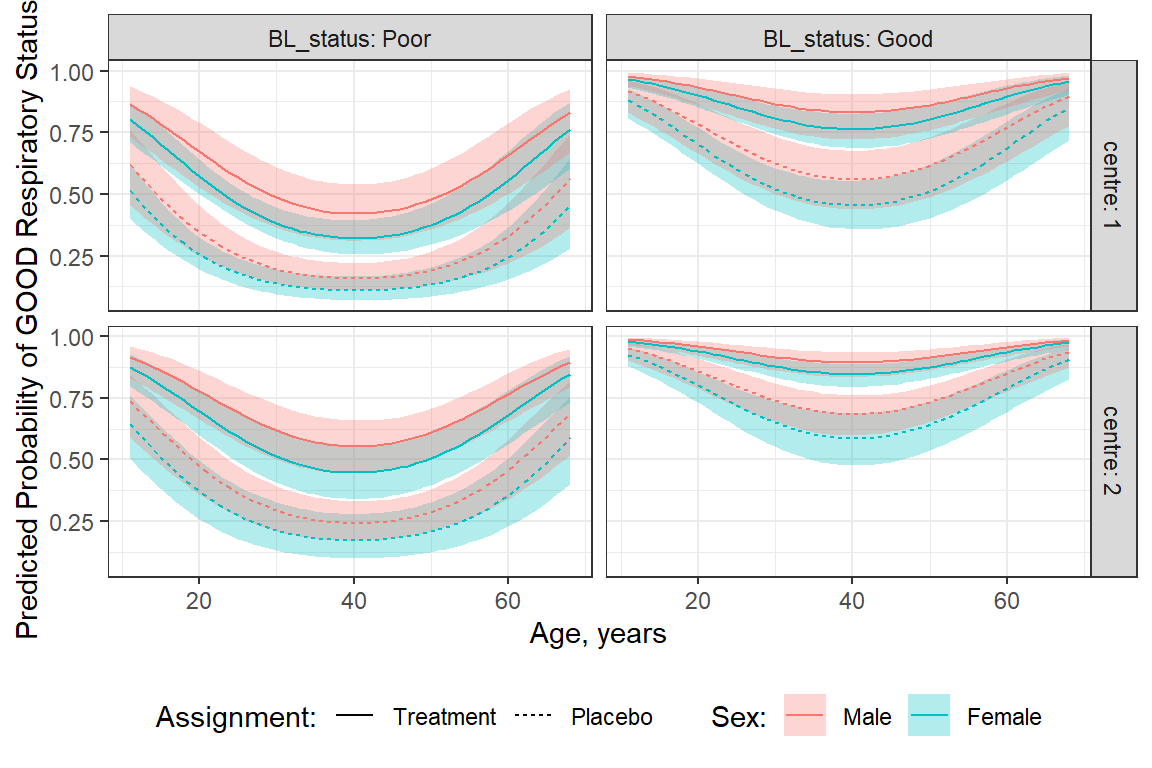

16.3.8.3 Females in Center 1

This example uses default settings.

interactions::interact_plot(model = fit_geeglm_ex,
                            pred = age,
                            modx = treatment,
                            mod2 = BL_status)  +
  theme_bw()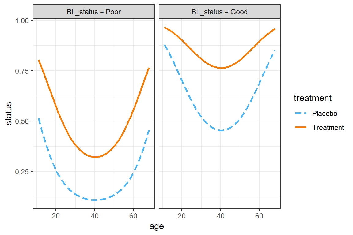

interactions::interact_plot(model = fit_geeglm_ex,
                            pred = age,
                            modx = treatment,
                            mod2 = BL_status,
                            at = list(sex = "Female",
                                      centre = "1"))  +
  theme_bw()

16.3.8.4 Males in Center 2

This example is more preped for publication.

interactions::interact_plot(model = fit_geeglm_ex,
                            pred = age,
                            modx = treatment,
                            mod2 = BL_status,
                            at = list(sex = "Male",
                                      centre = "2"),
                            x.label = "Age in Years",
                            y.label = "Predicted Probability of 'Good' Respiratory Status",
                            legend.main = "Intervention: ",
                            mod2.labels = c("Poor at Baseline",
                                            "Good at Baseline"),
                            colors = rep("black", times = 2)) +
  theme_bw() +
  theme(legend.position = c(1, 0),
        legend.justification = c(1.1, -0.1),
        legend.background = element_rect(color = "black"),
        legend.key.width = unit(1.5, "cm")) +
  labs(caption = "Note: Probibilities shown are specific to males at center 2")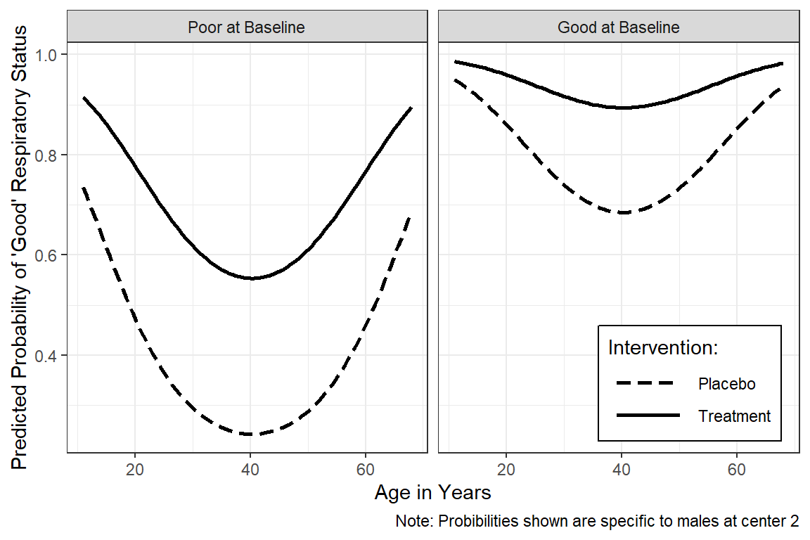

fit_geeglm_ex %>% 
  emmeans::emmeans(~ centre + treatment + sex + age + BL_status,
                   at = list(age = seq(from = 11, to = 68, by = 1),
                             sex = "Male",
                             centre = "2"),
                   type = "response",
                   level = .68) %>% 
  data.frame() %>% 
  ggplot(aes(x = age,
             y = prob,
             group = interaction(sex, treatment))) +
  geom_ribbon(aes(ymin = lower.CL,
                  ymax = upper.CL),
              alpha = .2) +
  geom_line(aes(linetype = fct_rev(treatment))) +
  theme_bw() + 
  facet_grid(~ BL_status) +
  labs(x = "Age, years",
       y = "Predicted Probability of\nGOOD Respiratory Status",
       color = "Sex:",
       fill = "Sex:",
       linetype = "Assignment:") +
  theme(legend.position = "bottom")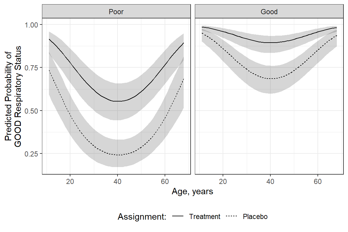

16.4 Conclusion

The Research Question

The question of interest is to assess whether the treatment is effective and to estimate its effect.

The Conclusion

After accounting for baseline status, age, sex and center, participants in the active treatment group had nearly four times higher odds of having ‘good’ respiratory status, when compared to the placebo, exp(b) = 3.881, p<.001, 95% CI [1.85, 8.14].