8 MLM, Centering/Scaling: Student Popularity

Download/install a new GitHub package
install.packages("devtools")
devtools::install_github("sarbearschwartz/apaSupp") # updated 9/17/2025
Load/activate these packages
library(haven)
library(tidyverse)
library(flextable)
library(apaSupp)      # Not on CRAN, on GitHub (see above)
library(lme4)
library(lmerTest)
library(optimx)
8.1 Background
The text “Multilevel Analysis: Techniques and Applications, Third Edition” (Hox, Moerbeek, and Van de Schoot 2017) has a companion website which includes links to all the data files used throughout the book (housed on the book’s GitHub repository).
The following example is used through out Hox, Moerbeek, and Van de Schoot (2017)’s chapater 2.
From Appendix E:
The popularity data in popular2.sav are simulated data for 2000 pupils in 100 schools. The purpose is to offer a very simple example for multilevel regression analysis. The main outcome variable is the pupil popularity, a popularity rating on a scale of 1-10 derived by a sociometric procedure. Typically, a sociometric procedure asks all pupils in a class to rate all the other pupils, and then assigns the average received popularity rating to each pupil. Because of the sociometric procedure, group effects as apparent from higher level variance components are rather strong. There is a second outcome variable: pupil popularity as rated by their teacher, on a scale from 1-10. The explanatory variables are pupil gender (boy=0, girl=1), pupil extraversion (10-point scale) and teacher experience in years. The popularity data have been generated to be a ‘nice’ well-behaved data set: the sample sizes at both levels are sufficient, the residuals have a normal distribution, and the multilevel effects are strong.

data_raw <- haven::read_sav("data/popular2.sav") %>%
  haven::as_factor() %>%              # retain the labels from SPSS --> factor
  haven::zap_label() %>%
  haven::zap_widths()
data_pop <- data_raw %>%
dplyr::mutate(id = paste(class, pupil,
sep = "_") %>% # create a unique id for each student (char)
factor()) %>% # declare id is a factor
dplyr::select(id, pupil:popteach) # reduce the variables includedRows: 2,000
Columns: 8
$ id <fct> 1_1, 1_2, 1_3, 1_4, 1_5, 1_6, 1_7, 1_8, 1_9, 1_10, 1_11, 1_12…
$ pupil <dbl> 1, 2, 3, 4, 5, 6, 7, 8, 9, 10, 11, 12, 13, 14, 15, 16, 17, 18…
$ class <dbl> 1, 1, 1, 1, 1, 1, 1, 1, 1, 1, 1, 1, 1, 1, 1, 1, 1, 1, 1, 1, 2…
$ extrav <dbl> 5, 7, 4, 3, 5, 4, 5, 4, 5, 5, 5, 5, 5, 5, 5, 6, 4, 4, 7, 4, 8…
$ sex <fct> girl, boy, girl, girl, girl, boy, boy, boy, boy, boy, girl, g…
$ texp <dbl> 24, 24, 24, 24, 24, 24, 24, 24, 24, 24, 24, 24, 24, 24, 24, 2…
$ popular <dbl> 6.3, 4.9, 5.3, 4.7, 6.0, 4.7, 5.9, 4.2, 5.2, 3.9, 5.7, 4.8, 5…
$ popteach <dbl> 6, 5, 6, 5, 6, 5, 5, 5, 5, 3, 5, 5, 5, 6, 5, 5, 2, 3, 7, 4, 6…data_pop %>%
ggplot() +
aes(x = extrav,
y = popular,
group = class) +
geom_smooth(method = "lm",
se = FALSE,
color = "black",
size = .2) +
theme_bw() +
geom_vline(xintercept = 0,
color = "red") +
labs(title = "OLS: Single Level Regression",
subtitle = "Thin black lines are OLS regression ran independently on each class",
x = "Student's Extroversion, as rated by their teacher",
y = "Student's Populartity, mean rating by their peers") +
coord_cartesian(xlim = c(0, 10),
ylim = c(0, 10)) +
scale_x_continuous(breaks = seq(from = 0, to = 10, by = 2)) +
scale_y_continuous(breaks = seq(from = 0, to = 10, by = 2))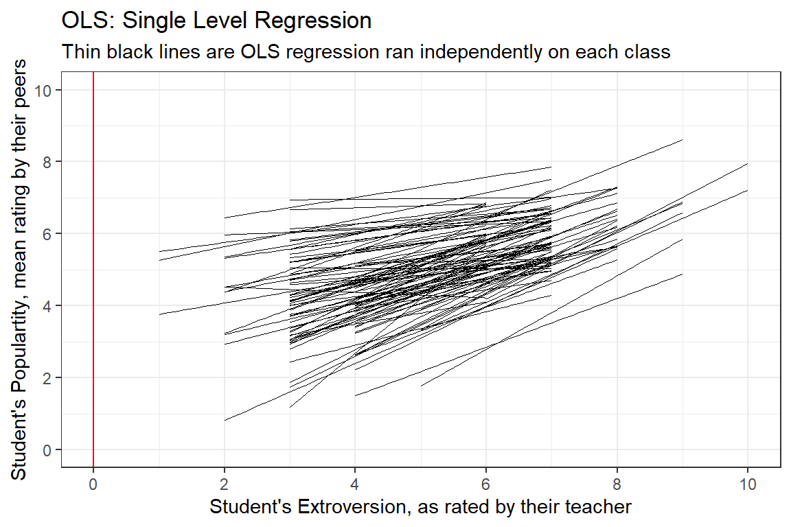
8.2 Grand-Mean-Centering and Standardizing Variables
It is best to manually determine the variable’s mean (mean()) and standard deviation (sd()).
[1] 5.215[1] 1.2623688.2.2 Standardizing
\[ VAR_Z = \frac{VAR - mean(VAR)}{sd(VAR)} \]
data_pop <- data_pop %>%
  dplyr::mutate(extravG =  extrav - 5.215) %>%
  dplyr::mutate(extravZ = (extrav - 5.215) / 1.262368)
data_pop %>%
dplyr::select("Original" = extrav,
"Centered" = extravG,
"Standardized" = extravZ) %>%
apaSupp::tab_desc(caption = "Descriptive statistics: Three versions of Extraversion")NA | M | SD | min | Q1 | Mdn | Q3 | max | |
|---|---|---|---|---|---|---|---|---|
Original | 0 | 5.21 | 1.26 | 1.00 | 4.00 | 5.00 | 6.00 | 10.00 |
Centered | 0 | 0.00 | 1.26 | -4.21 | -1.21 | -0.21 | 0.79 | 4.79 |
Standardized | 0 | 0.00 | 1.00 | -3.34 | -0.96 | -0.17 | 0.62 | 3.79 |
Note. N = 2000. NA = not available or missing; Mdn = median; Q1 = 25th percentile; Q3 = 75th percentile. | ||||||||
8.3 RI = ONLY Random Intercepts
8.3.1 Fit MLM with all 3 versions of the predictor
pop_lmer_1_raw <- lmerTest::lmer(popular ~ extrav + (1|class),
                                 data = data_pop,
                                 REML = FALSE)

pop_lmer_1_cen <- lmerTest::lmer(popular ~ extravG + (1|class),
                                 data = data_pop,
                                 REML = FALSE)

pop_lmer_1_std <- lmerTest::lmer(popular ~ extravZ + (1|class),
                                 data = data_pop,
REML = FALSE)apaSupp::tab_lmers(list("Original" = pop_lmer_1_raw,
"Centered" = pop_lmer_1_cen,
"Standardized" = pop_lmer_1_std),
narrow = TRUE,
caption = "MLM - RI: Effect of Grand-Mean Centering and Standardizing",
general_note = "The extraversion variable is on different scales.")
| Original | Centered | Standardized | |||
|---|---|---|---|---|---|---|
Variable | b | (SE) | b | (SE) | b | (SE) |
(Intercept) | 2.54 | (0.14) *** | 5.08 | (0.09) *** | 5.08 | (0.09) *** |
extrav | 0.49 | (0.02) *** | ||||
extravG | 0.49 | (0.02) *** | ||||
extravZ | 0.61 | (0.03) *** | ||||
class.var__(Intercept) | 0.83 | 0.83 | 0.83 | |||
Residual.var__Observation | 0.93 | 0.93 | 0.93 | |||
AIC | 5,832 | 5,832 | 5,832 | |||
BIC | 5,854 | 5,854 | 5,854 | |||
Log-likelihood | -2,912 | -2,912 | -2,912 | |||
Note. The extraversion variable is on different scales. | ||||||
* p < .05. ** p < .01. *** p < .001. | ||||||
** MLM - Random Intercepts ONLY**
- Grand-Mean Centering a Predictor
-
Different than when using the Raw Predictor:
-
fixed intercept
-
Same as when using the Raw Predictor:
-
fixed estimates or slopes for all predictors (main effects and interactions)
-
random estimates, i.e. variance and covariance components, includin the residual variance
-
model fit statistics, including AIC, BIC, and the Log Loikelihood (-2LL or deviance)
- Standardize a Predictor
-
Different than when using the Raw Predictor:
-
fixed intercept (same as if using the grand-mean centered predictor)
-
fixed estimate (slope) for that variable
-
Stays the SAME:
-
random estimates, i.e. variance and covariance components, includin the residual variance
-
model fit statistics, including AIC, BIC, and the Log Loikelihood (-2LL or deviance)
8.3.1.1 Fixed Effects: intercept and slope
There is only ONE fixed intercept and ONE fixed slope.
The fixef() function extracts the estimates of the fixed effects.
(Intercept)      extrav
2.5427027 0.4862002 [1] 2.542703[1] 0.4862002data_pop %>%
ggplot() +
aes(x = extrav,
y = popular,
group = class) +
geom_smooth(method = "lm",
se = FALSE,
color = "black",
size = .2) +
geom_abline(intercept = fixef(pop_lmer_1_raw)[["(Intercept)"]],
slope = fixef(pop_lmer_1_raw)[["extrav"]],
color = "hot pink",
size = 2) +
theme_bw() +
geom_vline(xintercept = 0,
color = "red") +
labs(title = "MLM-RI: Extroversion = raw score",
subtitle = "Thin black lines are OLS regression ran independently on each class",
x = "Student's Extroversion, as rated by their teacher",
y = "Student's Populartity, mean rating by their peers") +
coord_cartesian(xlim = c(0, 10),
ylim = c(0, 10)) +
scale_x_continuous(breaks = seq(from = 0, to = 10, by = 2)) +
scale_y_continuous(breaks = seq(from = 0, to = 10, by = 2))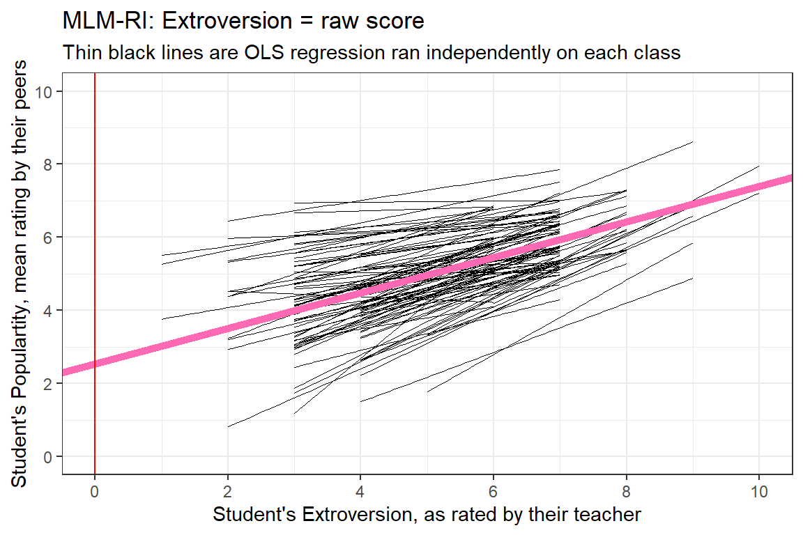
8.3.1.2 Random Effects: intercepts
There is a different random intercept for EACH CLASS. These tell how far each class’s average is off of the grand average.
The ranef() function extracts the random effects from a fitted model object
List of 1
 $ class:'data.frame':  100 obs. of  1 variable:
  ..$ (Intercept): num [1:100] 0.165 -0.7536 -0.3646 0.5405 -0.0994 ...
  ..- attr(*, "postVar")= num [1, 1, 1:100] 0.044 0.044 0.0486 0.0386 0.042 ...
- attr(*, "class")= chr "ranef.mer" (Intercept)
1 0.16499938
2 -0.75362983
3 -0.36464658
4 0.54049206
5 -0.09943663
6 -0.60487822ranef(pop_lmer_1_raw)$class %>%
dplyr::rename(Random_Intercepts = "(Intercept)") %>%
apaSupp::spicy_histos(Random_Intercepts)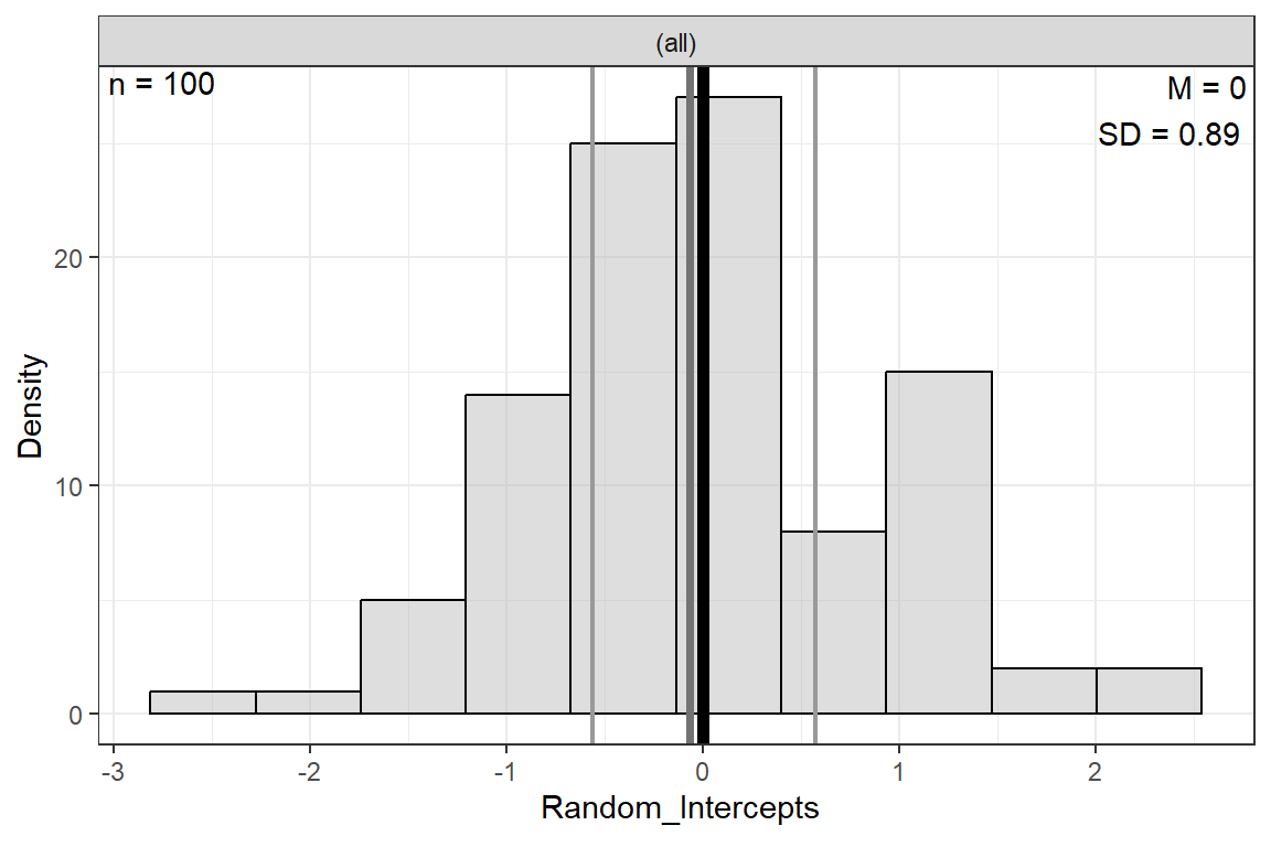
8.3.1.3 Predictions
 Named num [1:2000] 5.14 6.11 4.65 4.17 5.14 ...
- attr(*, "names")= chr [1:2000] "1" "2" "3" "4" ... 1 2 3 4 5 6
5.138703 6.111103 4.652503 4.166303 5.138703 4.652503 data_pop %>%
dplyr::mutate(pred = predict(pop_lmer_1_raw)) %>%
ggplot(aes(x = extrav,
y = pred,
group = class)) +
geom_line(size = .2) +
geom_abline(intercept = fixef(pop_lmer_1_raw)[["(Intercept)"]],
slope = fixef(pop_lmer_1_raw)[["extrav"]],
color = "hot pink",
size = 2) +
theme_bw() +
geom_vline(xintercept = 0,
color = "red") +
geom_vline(xintercept = 5.215,
color = "blue") +
labs(title = "MLM-RI: Extroversion = raw score",
subtitle = "Thin black lines are group-wise predictions, one per class",
x = "Student's Extroversion, as rated by their teacher",
y = "Predicted\nStudent's Populartity, mean rating by their peers") +
coord_cartesian(xlim = c(0, 10),
ylim = c(0, 10)) +
scale_x_continuous(breaks = seq(from = 0, to = 10, by = 2)) +
scale_y_continuous(breaks = seq(from = 0, to = 10, by = 2))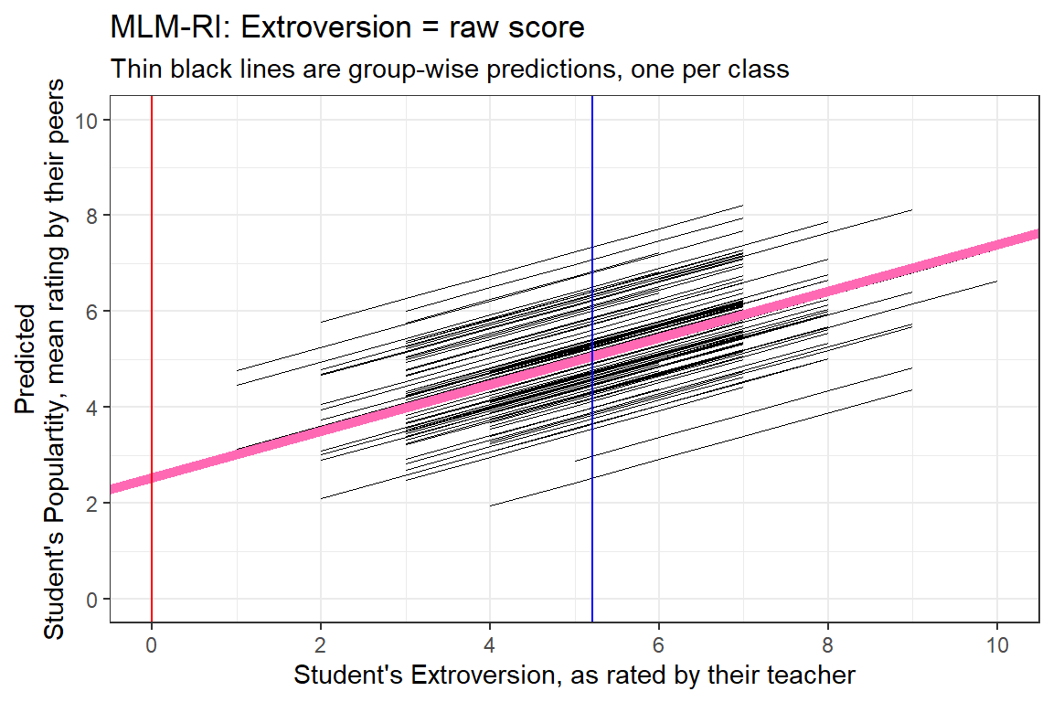
8.3.1.4 Combined Effects
The coef() function computes the sum of the random and fixed effects coefficients for each explanatory variable for each level of each grouping factor.
List of 1
 $ class:'data.frame':  100 obs. of  2 variables:
  ..$ (Intercept): num [1:100] 2.71 1.79 2.18 3.08 2.44 ...
  ..$ extrav     : num [1:100] 0.486 0.486 0.486 0.486 0.486 ...
- attr(*, "class")= chr "coef.mer" (Intercept) extrav
1 2.707702 0.4862002
2 1.789073 0.4862002
3 2.178056 0.4862002
4 3.083195 0.4862002
5 2.443266 0.4862002
6 1.937824 0.4862002data_pop %>%
dplyr::mutate(pred = predict(pop_lmer_1_raw)) %>%
ggplot() +
aes(x = extrav,
y = pred,
group = class) +
geom_rect(aes(xmin = 0 - 0.25,
xmax = 0 + 0.25,
ymin = fixef(pop_lmer_1_raw)[["(Intercept)"]]- 2.5,
ymax = fixef(pop_lmer_1_raw)[["(Intercept)"]]+ 2.5),
fill = "yellow",
alpha = 0.05) +
geom_abline(data = coef(pop_lmer_1_raw)$class %>% dplyr::rename(Intercept = "(Intercept)"),
aes(intercept = Intercept,
slope = extrav),
color = "gray",
size = .1) +
geom_line(size = .2) +
geom_abline(intercept = fixef(pop_lmer_1_raw)[["(Intercept)"]],
slope = fixef(pop_lmer_1_raw)[["extrav"]],
color = "hot pink",
size = 2) +
theme_bw() +
geom_vline(xintercept = 0,
color = "red") +
geom_vline(xintercept = 5.215,
color = "blue") +
labs(title = "MLM-RI: Extroversion = raw score",
subtitle = "Thin black lines are group-wise predictions, one per class EXTRAPOLATED OUT",
x = "Student's Extroversion, as rated by their teacher",
y = "Predicted\nStudent's Populartity, mean rating by their peers") +
coord_cartesian(xlim = c(0, 10),
ylim = c(0, 10)) +
scale_x_continuous(breaks = seq(from = 0, to = 10, by = 2)) +
scale_y_continuous(breaks = seq(from = 0, to = 10, by = 2)) 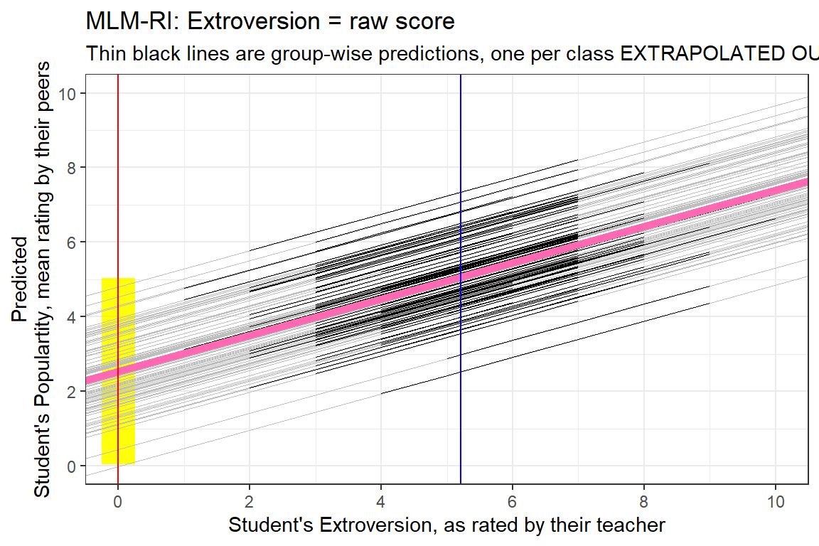
8.3.2 Comapre the Centered Version
data_pop %>%
  dplyr::mutate(pred = predict(pop_lmer_1_cen)) %>%
  ggplot() +
  aes(x = extravG,
      y = pred,
      group = class) +
  geom_rect(aes(xmin = -5.215 - 0.25,
                xmax = -5.215 + 0.25,
                ymin = fixef(pop_lmer_1_raw)[["(Intercept)"]]- 2.5,
                ymax = fixef(pop_lmer_1_raw)[["(Intercept)"]]+ 2.5),
            fill = "yellow",
            alpha = 0.05) +
  geom_rect(aes(xmin = 0 - 0.25,
                xmax = 0 + 0.25,
                ymin = fixef(pop_lmer_1_cen)[["(Intercept)"]]- 2.5,
                ymax = fixef(pop_lmer_1_cen)[["(Intercept)"]]+ 2.5),
            fill = "yellow",
            alpha = 0.05) +
  geom_abline(data = coef(pop_lmer_1_cen)$class %>% dplyr::rename(Intercept = "(Intercept)"),
              aes(intercept = Intercept,
                  slope     = extravG),
              color = "gray",
              size = .1) +
  geom_line(size = .2) +
  geom_abline(intercept = fixef(pop_lmer_1_cen)[["(Intercept)"]],
              slope     = fixef(pop_lmer_1_cen)[["extravG"]],
              color = "hot pink",
              size = 2) +
  theme_bw() +
  geom_vline(xintercept = -5.215,
             color = "blue") +
  geom_vline(xintercept = 0,
             color = "red") +
  labs(title = "MLM-RI: Extroversion = grand-mean centered",
       subtitle = "Thin black lines are group-wise predictions, one per class EXTRAPOLATED OUT",
       x = "GRAND-MEAN CENTERED Student's Extroversion, as rated by their teacher",
       y = "Predicted\nStudent's Populartity, mean rating by their peers") +
  coord_cartesian(xlim = c(-5, 5),
                  ylim = c(0, 10)) +
  scale_x_continuous(breaks = seq(from = -4, to =  4, by = 2)) +
  scale_y_continuous(breaks = seq(from =  0, to = 10, by = 2))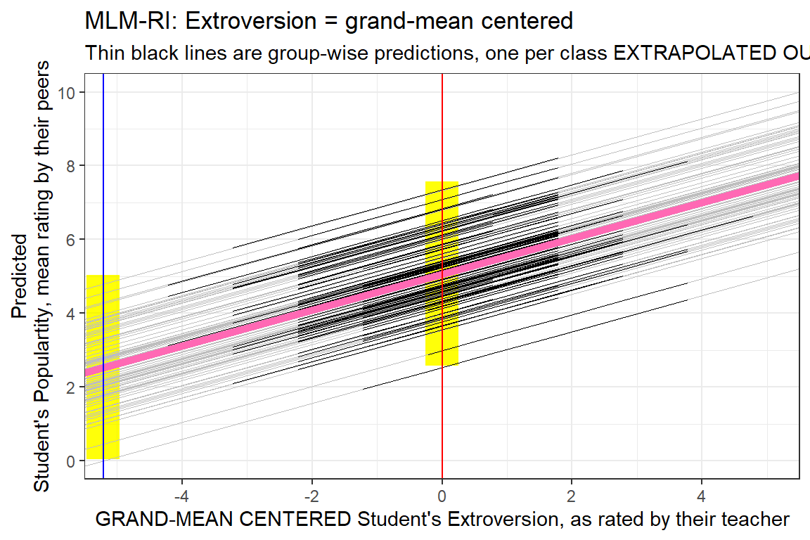
8.3.3 Comapre the Standardized Version
data_pop %>%
  dplyr::mutate(pred = predict(pop_lmer_1_std)) %>%
  ggplot() +
  aes(x = extravZ,
      y = pred,
      group = class) +
  geom_rect(aes(xmin = 0 - 0.25,
                xmax = 0 + 0.25,
                ymin = fixef(pop_lmer_1_cen)[["(Intercept)"]]- 2.5,
                ymax = fixef(pop_lmer_1_cen)[["(Intercept)"]]+ 2.5),
            fill = "yellow",
            alpha = 0.05) +
  geom_abline(data = coef(pop_lmer_1_std)$class %>% dplyr::rename(Intercept = "(Intercept)"),
              aes(intercept = Intercept,
                  slope     = extravZ),
              color = "gray",
              size = .1) +
  geom_line(size = .2) +
  geom_abline(intercept = fixef(pop_lmer_1_std)[["(Intercept)"]],
              slope     = fixef(pop_lmer_1_std)[["extravZ"]],
              color = "hot pink",
              size = 2) +
  theme_bw() +
  geom_vline(xintercept = 0,
             color = "red") +
  geom_vline(xintercept = -5.215,
             color = "blue") +
  labs(title = "MLM-RI: Extroversion = standardized",
       subtitle = "Thin black lines are group-wise predictions, one per class EXTRAPOLATED OUT",
       x = "STANDARDIZED Student's Extroversion, as rated by their teacher",
       y = "Predicted\nStudent's Populartity, mean rating by their peers") +
  coord_cartesian(xlim = c(-5, 5),
                  ylim = c(0, 10)) +
  scale_x_continuous(breaks = seq(from = -4, to =  4, by = 2)) +
  scale_y_continuous(breaks = seq(from =  0, to = 10, by = 2))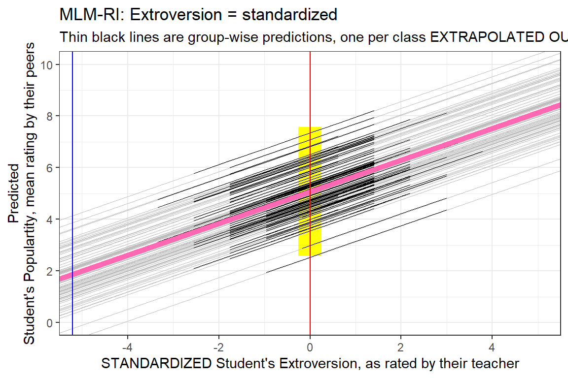
8.4 RIAS = Random Intercepts AND Slopes
8.4.1 Fit MLM with all 3 versions of the predictor
pop_lmer_2_raw <- lmerTest::lmer(popular ~ extrav + (extrav|class),
                                 data = data_pop,
                                 control = lmerControl(optimizer = "Nelder_Mead"),
                                 REML = FALSE)

pop_lmer_2_cen <- lmerTest::lmer(popular ~ extravG + (extravG|class),
                                 data = data_pop,
                                 REML = FALSE)

pop_lmer_2_std <- lmerTest::lmer(popular ~ extravZ + (extravZ|class),
                                 data = data_pop,
REML = FALSE)apaSupp::tab_lmers(list("Original" = pop_lmer_2_raw,
"Centered" = pop_lmer_2_cen,
"Standardized" = pop_lmer_2_std),
narrow = TRUE,
caption = "MLM - RIAS: Effect of Grand-Mean Centering and Standardizing")
| Original | Centered | Standardized | |||
|---|---|---|---|---|---|---|
Variable | b | (SE) | b | (SE) | b | (SE) |
(Intercept) | 2.46 | (0.20) *** | 5.03 | (0.10) *** | 5.03 | (0.10) *** |
extrav | 0.49 | (0.03) *** | ||||
extravG | 0.49 | (0.03) *** | ||||
extravZ | 0.62 | (0.03) *** | ||||
class.var__(Intercept) | 2.95 | 0.88 | 0.88 | |||
class.cov__(Intercept).extrav | -0.26 | |||||
class.var__extrav | 0.03 | |||||
Residual.var__Observation | 0.90 | 0.90 | 0.90 | |||
class.cov__(Intercept).extravG | -0.13 | |||||
class.var__extravG | 0.03 | |||||
class.cov__(Intercept).extravZ | -0.17 | |||||
class.var__extravZ | 0.04 | |||||
AIC | 5,783 | 5,783 | 5,783 | |||
BIC | 5,816 | 5,816 | 5,816 | |||
Log-likelihood | -2,885 | -2,885 | -2,885 | |||
Note. | ||||||
* p < .05. ** p < .01. *** p < .001. | ||||||
** MLM - Random Intercepts AND Slopes**
- Grand-Mean Centering a Predictor
-
Different than when using the Raw Predictor:
-
fixed intercept
-
random estimates, i.e. variance and covariance components, includin the residual variance
-
Same as when using the Raw Predictor:
-
fixed estimates or slopes for all predictors (main effects and interactions)
-
model fit statistics, including AIC, BIC, and the Log Loikelihood (-2LL or deviance)
- Standardize a Predictor
-
Different than when using the Raw Predictor:
-
fixed intercept (same as if using the grand-mean centered predictor)
-
fixed estimate (slope) for that variable
-
random estimates, i.e. variance and covariance components, includin the residual variance
-
Stays the SAME:
-
model fit statistics, including AIC, BIC, and the Log Loikelihood (-2LL or deviance)
8.4.1.1 Fixed Effects: intercept and slope
There is only ONE fixed intercept and ONE fixed slope.
The fixef() function extracts the estimates of the fixed effects.
(Intercept)      extrav
2.4613507 0.4929021 [1] 2.461351[1] 0.4929021data_pop %>%
ggplot() +
aes(x = extrav,
y = popular,
group = class) +
geom_smooth(method = "lm",
se = FALSE,
color = "black",
size = .2) +
geom_abline(intercept = fixef(pop_lmer_2_raw)[["(Intercept)"]],
slope = fixef(pop_lmer_2_raw)[["extrav"]],
color = "hot pink",
size = 2) +
theme_bw() +
geom_vline(xintercept = 0,
color = "red") +
geom_vline(xintercept = 5.215,
color = "blue") +
labs(title = "MLM-RIAS: Extroversion = raw score",
subtitle = "Thin black lines are OLS regression ran independently on each class",
x = "Student's Extroversion, as rated by their teacher",
y = "Student's Populartity, mean rating by their peers") +
coord_cartesian(xlim = c(0, 10),
ylim = c(0, 10)) +
scale_x_continuous(breaks = seq(from = 0, to = 10, by = 2)) +
scale_y_continuous(breaks = seq(from = 0, to = 10, by = 2))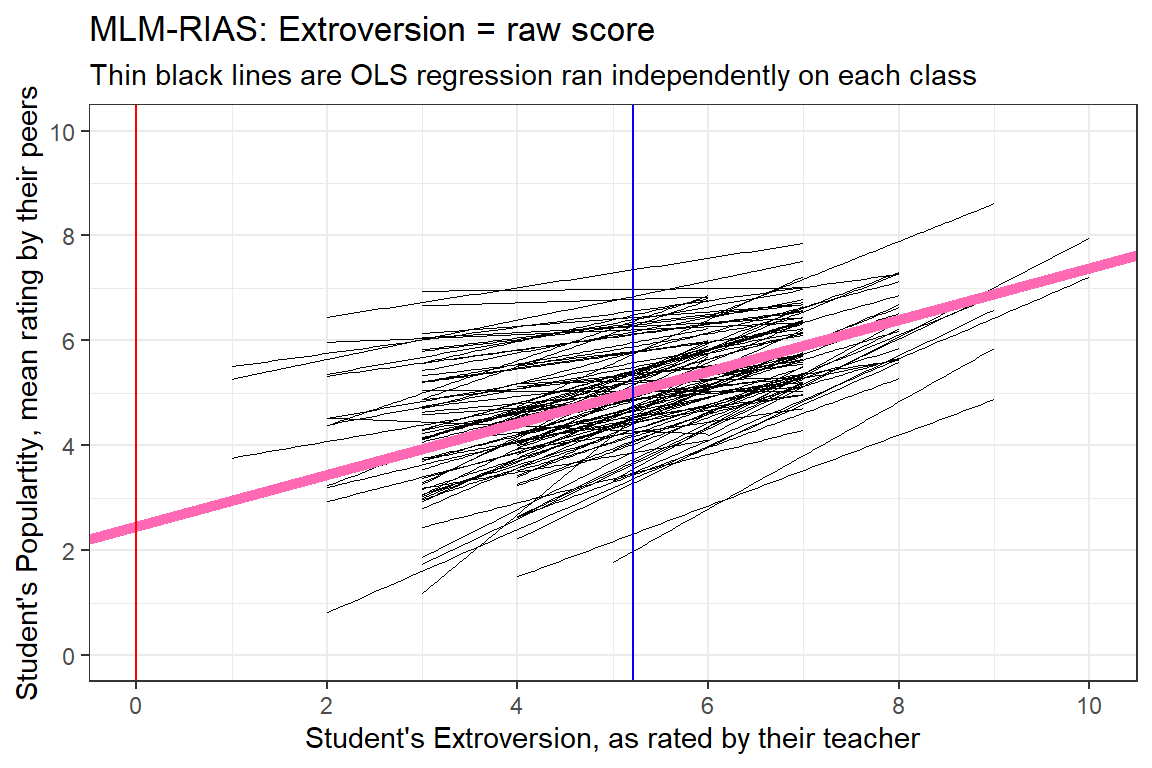
8.4.1.2 Random Effects: intercepts
There is a different random intercept AND random slope for EACH CLASS. These tell how far each class’s average is off of the grand average AND how far each class’s slope is off of the grand average sope.
The ranef() function extracts the random effects from a fitted model object
List of 1
 $ class:'data.frame':  100 obs. of  2 variables:
  ..$ (Intercept): num [1:100] 0.341 -1.18 -0.627 1.079 -0.191 ...
  ..$ extrav     : num [1:100] -0.0272 0.0974 0.0565 -0.0988 0.0208 ...
  ..- attr(*, "postVar")= num [1:2, 1:2, 1:100] 0.21331 -0.02975 -0.02975 0.00499 0.20573 ...
- attr(*, "class")= chr "ranef.mer" (Intercept) extrav
1 0.3412775 -0.02721141
2 -1.1800363 0.09737325
3 -0.6268925 0.05654028
4 1.0791076 -0.09876691
5 -0.1910473 0.02083052
6 -0.9833298 0.08369928ranef(pop_lmer_2_raw)$class %>%
dplyr::rename(Random_Intercepts = "(Intercept)") %>%
apaSupp::spicy_histos(Random_Intercepts)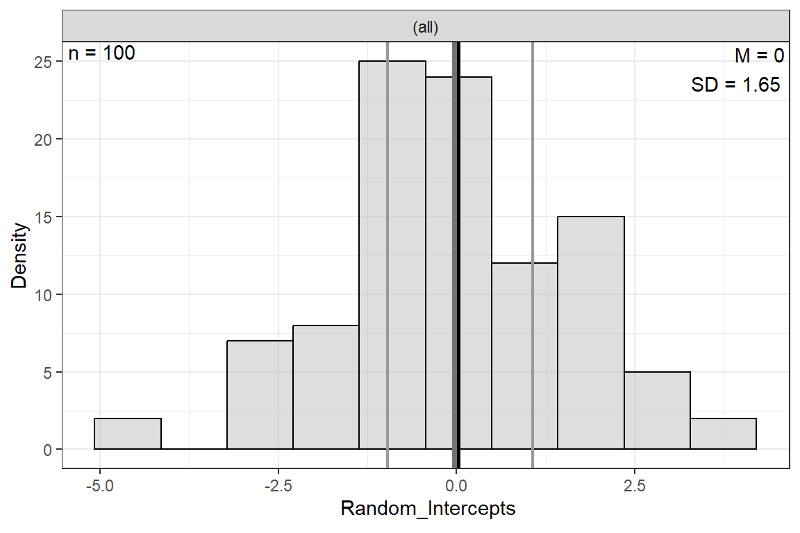
8.4.1.3 Predictions
 Named num [1:2000] 5.13 6.06 4.67 4.2 5.13 ...
- attr(*, "names")= chr [1:2000] "1" "2" "3" "4" ... 1 2 3 4 5 6
5.131082 6.062463 4.665391 4.199700 5.131082 4.665391 data_pop %>%
dplyr::mutate(pred = predict(pop_lmer_2_raw)) %>%
ggplot(aes(x = extrav,
y = pred,
group = class)) +
geom_line(size = .2) +
geom_abline(intercept = fixef(pop_lmer_2_raw)[["(Intercept)"]],
slope = fixef(pop_lmer_2_raw)[["extrav"]],
color = "hot pink",
size = 2) +
theme_bw() +
geom_vline(xintercept = 0,
color = "red") +
geom_vline(xintercept = 5.215,
color = "blue") +
labs(title = "MLM-RIAS: Extroversion = raw score",
subtitle = "Thin black lines are group-wise predictions, one per class",
x = "Student's Extroversion, as rated by their teacher",
y = "Predicted\nStudent's Populartity, mean rating by their peers") +
coord_cartesian(xlim = c(0, 10),
ylim = c(0, 10)) +
scale_x_continuous(breaks = seq(from = 0, to = 10, by = 2)) +
scale_y_continuous(breaks = seq(from = 0, to = 10, by = 2))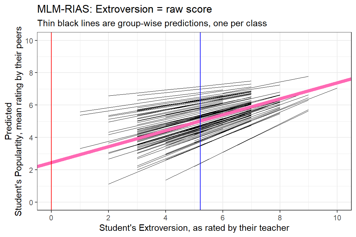
8.4.1.4 Combined Effects
The coef() function computes the sum of the random and fixed effects coefficients for each explanatory variable for each level of each grouping factor.
List of 1
 $ class:'data.frame':  100 obs. of  2 variables:
  ..$ (Intercept): num [1:100] 2.71 1.79 2.18 3.08 2.44 ...
  ..$ extrav     : num [1:100] 0.486 0.486 0.486 0.486 0.486 ...
- attr(*, "class")= chr "coef.mer" (Intercept) extrav
1 2.707702 0.4862002
2 1.789073 0.4862002
3 2.178056 0.4862002
4 3.083195 0.4862002
5 2.443266 0.4862002
6 1.937824 0.4862002data_pop %>%
dplyr::mutate(pred = predict(pop_lmer_2_raw)) %>%
ggplot() +
aes(x = extrav,
y = pred,
group = class) +
geom_rect(aes(xmin = 0 - 0.25,
xmax = 0 + 0.25,
ymin = fixef(pop_lmer_2_raw)[["(Intercept)"]]- 4.5,
ymax = fixef(pop_lmer_2_raw)[["(Intercept)"]]+ 4.5),
fill = "yellow",
alpha = 0.05) +
geom_abline(data = coef(pop_lmer_2_raw)$class %>% dplyr::rename(Intercept = "(Intercept)"),
aes(intercept = Intercept,
slope = extrav),
color = "gray",
size = .1) +
geom_line(size = .2) +
geom_abline(intercept = fixef(pop_lmer_2_raw)[["(Intercept)"]],
slope = fixef(pop_lmer_2_raw)[["extrav"]],
color = "hot pink",
size = 2) +
theme_bw() +
geom_vline(xintercept = 0,
color = "red") +
geom_vline(xintercept = 5.215,
color = "blue") +
labs(title = "MLM-RIAS: Extroversion = raw score",
subtitle = "Thin black lines are group-wise predictions, one per class EXTRAPOLATED OUT",
x = "Student's Extroversion, as rated by their teacher",
y = "Predicted\nStudent's Populartity, mean rating by their peers") +
coord_cartesian(xlim = c(0, 10),
ylim = c(0, 10)) +
scale_x_continuous(breaks = seq(from = 0, to = 10, by = 2)) +
scale_y_continuous(breaks = seq(from = 0, to = 10, by = 2)) 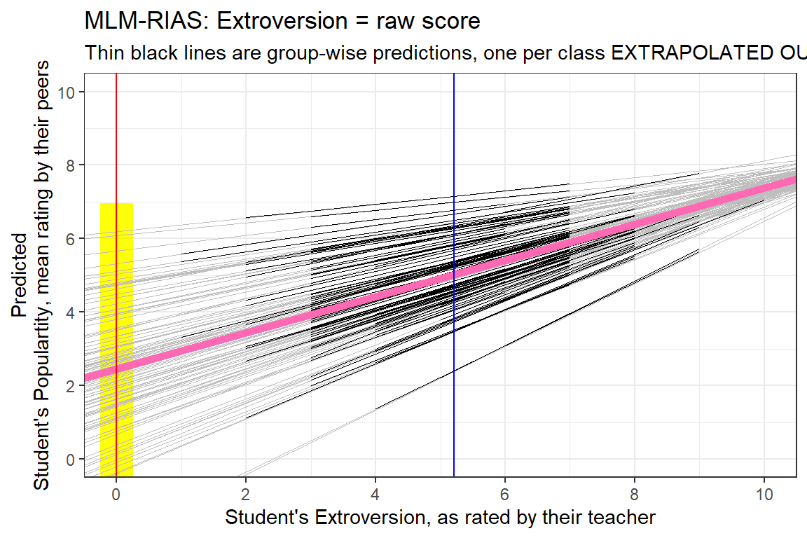
8.4.2 Comapre the Centered Version
data_pop %>%
  dplyr::mutate(pred = predict(pop_lmer_2_cen)) %>%
  ggplot() +
  aes(x = extravG,
      y = pred,
      group = class) +
  geom_rect(aes(xmin = -5.215 - 0.25,
                xmax = -5.215 + 0.25,
                ymin = fixef(pop_lmer_2_raw)[["(Intercept)"]]- 4.5,
                ymax = fixef(pop_lmer_2_raw)[["(Intercept)"]]+ 4.5),
            fill = "yellow",
            alpha = 0.05) +
  geom_rect(aes(xmin = 0 - 0.25,
                xmax = 0 + 0.25,
                ymin = fixef(pop_lmer_2_cen)[["(Intercept)"]]- 2.5,
                ymax = fixef(pop_lmer_2_cen)[["(Intercept)"]]+ 2.5),
            fill = "yellow",
            alpha = 0.05) +
  geom_abline(data = coef(pop_lmer_2_cen)$class %>% dplyr::rename(Intercept = "(Intercept)"),
              aes(intercept = Intercept,
                  slope     = extravG),
              color = "gray",
              size = .1) +
  geom_line(size = .2) +
  geom_abline(intercept = fixef(pop_lmer_2_cen)[["(Intercept)"]],
              slope     = fixef(pop_lmer_2_cen)[["extravG"]],
              color = "hot pink",
              size = 2) +
  theme_bw() +
  geom_vline(xintercept = -5.215,
             color = "blue") +
  geom_vline(xintercept = 0,
             color = "red") +
  labs(title = "MLM-RIAS: Extroversion = grand-mean centered",
       subtitle = "Thin black lines are group-wise predictions, one per class EXTRAPOLATED OUT",
       x = "GRAND-MEAN CENTERED Student's Extroversion, as rated by their teacher",
       y = "Predicted\nStudent's Populartity, mean rating by their peers") +
  coord_cartesian(xlim = c(-5, 5),
                  ylim = c(0, 10)) +
  scale_x_continuous(breaks = seq(from = -4, to =  4, by = 2)) +
  scale_y_continuous(breaks = seq(from =  0, to = 10, by = 2))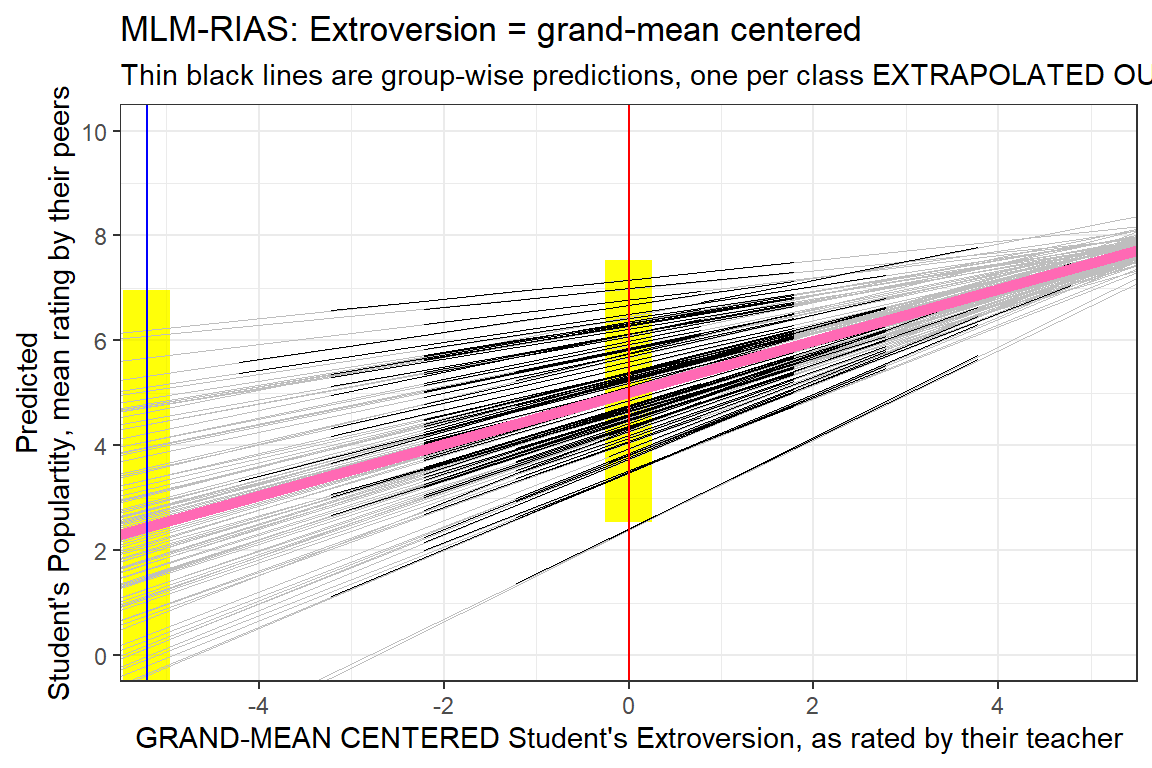
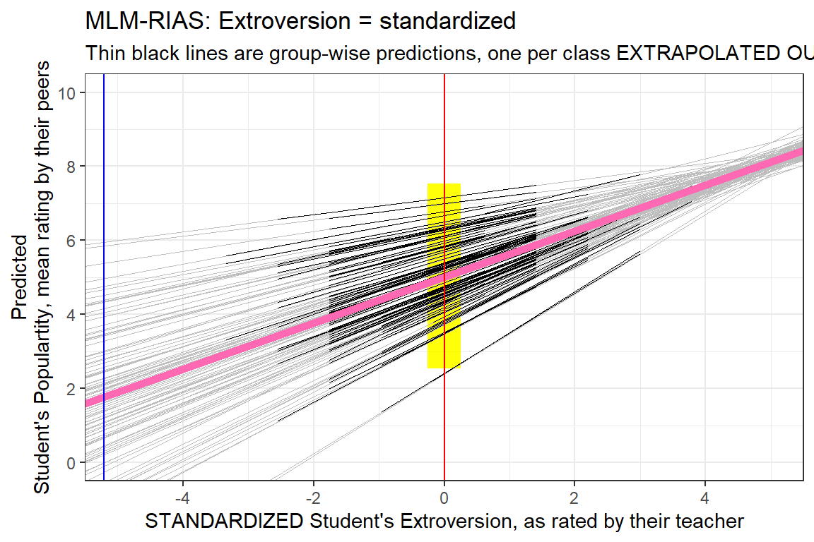
8.4.3 Compare the Standardized Version
data_pop %>%
  dplyr::mutate(pred = predict(pop_lmer_2_std)) %>%
  ggplot() +
  aes(x = extravZ,
      y = pred,
      group = class) +
  geom_rect(aes(xmin = 0 - 0.25,
                xmax = 0 + 0.25,
                ymin = fixef(pop_lmer_2_cen)[["(Intercept)"]]- 2.5,
                ymax = fixef(pop_lmer_2_cen)[["(Intercept)"]]+ 2.5),
            fill = "yellow",
            alpha = 0.05) +
  geom_abline(data = coef(pop_lmer_2_std)$class %>% dplyr::rename(Intercept = "(Intercept)"),
              aes(intercept = Intercept,
                  slope     = extravZ),
              color = "gray",
              size = .1) +
  geom_line(size = .2) +
  geom_abline(intercept = fixef(pop_lmer_2_std)[["(Intercept)"]],
              slope     = fixef(pop_lmer_2_std)[["extravZ"]],
              color = "hot pink",
              size = 2) +
  theme_bw() +
  geom_vline(xintercept = 0,
             color = "red") +
  geom_vline(xintercept = -5.215,
             color = "blue") +
  labs(title = "MLM-RIAS: Extroversion = standardized",
       subtitle = "Thin black lines are group-wise predictions, one per class EXTRAPOLATED OUT",
       x = "STANDARDIZED Student's Extroversion, as rated by their teacher",
       y = "Predicted\nStudent's Populartity, mean rating by their peers") +
  coord_cartesian(xlim = c(-5, 5),
                  ylim = c(0, 10)) +
  scale_x_continuous(breaks = seq(from = -4, to =  4, by = 2)) +
  scale_y_continuous(breaks = seq(from =  0, to = 10, by = 2))