23 GLMM, Count Outcome: Bolous

GLMM FAQ by: Ben Bolker and others

https://bbolker.github.io/mixedmodels-misc/glmmFAQ.html

23.1 Packages

23.1.1 CRAN

library(tidyverse)    # all things tidy
library(pander)       # nice looking genderal tabulations
library(furniture)    # nice table1() descriptives
library(texreg)       # Convert Regression Output to LaTeX or HTML Tables
library(psych)        # contains some useful functions, like headTail

library(lme4)         # Linear, generalized linear, & nonlinear mixed models
library(gee)          # Generalized Estimating Equations
library(optimx)       # Optimizers for use in lme4::glmer
library(MuMIn)        # Multi-Model Inference (caluclate QIC)
library(effects)      # Plotting estimated marginal means
library(interactions)
library(performance)

library(patchwork)    # combining graphics\


library(cold)   # this package holds the dataset we need

23.1.2 GitHub

Helper extract functions for exponentiating parameters form generalized regression models within a texreg table of model parameters.

# install.packages("devtools")
# library(devtools)
# install_github("SarBearSchwartz/texreghelpr")

library(texreghelpr)

23.2 Data Prep

Bolus data from Weiss 2005

Patient controlled analgesia (PCA) comparing 2 dosing regimes to self-control pain

The dataset has the number of requests per interval in 12 successive four-hourly intervals following abdominal surgery for 65 patients in a clinical trial to compare two groups (bolus/lock-out combinations).

Bolus= Large dose of medication given (usually intravenously by direct infusion injection or gravity drip) to raise blood-level concentrations to a therapeutic level

A ‘lock-out’ period followed each dose, where subject may not administer more medication.

Lock-out time is twice as long in 2mg/dose group
Allows for max of 30 dosages in 2mg/dose and 60 in 1mg/dose group in any 4-hour period
No responses neared these upper limits

Variable List:

Indicators
id unique subject indicator
time 11 consecutive 4-hour periods: 0, 1, 2, …, 10
Outcome or dependent variable
count # doses recorded for in that 4-hour period
Main predictor or independent variable of interest
group1mg/dose group, 2mg/dose group

23.2.1 Import

data("bolus", package = "cold")

df_raw <- bolus

str(df_raw) # see the structure

'data.frame':   780 obs. of  4 variables:
 $ id   : int  1 1 1 1 1 1 1 1 1 1 ...
 $ group: Factor w/ 2 levels "1mg","2mg": 2 2 2 2 2 2 2 2 2 2 ...
 $ time : int  1 2 3 4 5 6 7 8 9 10 ...
 $ y    : int  5 2 2 5 2 4 0 2 4 4 ...

psych::headTail(df_raw)

     id group time   y
1     1   2mg    1   5
2     1   2mg    2   2
3     1   2mg    3   2
4     1   2mg    4   5
... ...  <NA>  ... ...
777  65   1mg    9   6
778  65   1mg   10   1
779  65   1mg   11   2
780  65   1mg   12   0

23.2.2 Long Format

df_long <- df_raw %>% 
  dplyr::rename(count = y) %>% 
  dplyr::mutate(id = factor(id)) %>% 
  dplyr::mutate(time = time - 1) %>% 
  dplyr::mutate(timeF = factor(time)) %>% 
  dplyr::mutate(group = factor(group))

str(df_long) # see the structure

'data.frame':   780 obs. of  5 variables:
 $ id   : Factor w/ 65 levels "1","2","3","4",..: 1 1 1 1 1 1 1 1 1 1 ...
 $ group: Factor w/ 2 levels "1mg","2mg": 2 2 2 2 2 2 2 2 2 2 ...
 $ time : num  0 1 2 3 4 5 6 7 8 9 ...
 $ count: int  5 2 2 5 2 4 0 2 4 4 ...
 $ timeF: Factor w/ 12 levels "0","1","2","3",..: 1 2 3 4 5 6 7 8 9 10 ...

psych::headTail(df_long)

      id group time count timeF
1      1   2mg    0     5     0
2      1   2mg    1     2     1
3      1   2mg    2     2     2
4      1   2mg    3     5     3
... <NA>  <NA>  ...   ...  <NA>
777   65   1mg    8     6     8
778   65   1mg    9     1     9
779   65   1mg   10     2    10
780   65   1mg   11     0    11

23.2.3 Wide Format

df_wide <- df_long %>% 
  dplyr::select(-timeF) %>%
  tidyr::pivot_wider(names_from = time,
                     names_prefix = "time_",
                     values_from = count)

str(df_wide) # see the structure

tibble [65 × 14] (S3: tbl_df/tbl/data.frame)
 $ id     : Factor w/ 65 levels "1","2","3","4",..: 1 2 3 4 5 6 7 8 9 10 ...
 $ group  : Factor w/ 2 levels "1mg","2mg": 2 2 2 2 2 2 2 2 2 2 ...
 $ time_0 : int [1:65] 5 5 6 4 8 10 2 14 7 3 ...
 $ time_1 : int [1:65] 2 3 4 1 7 6 4 2 10 0 ...
 $ time_2 : int [1:65] 2 5 8 4 7 5 7 10 9 7 ...
 $ time_3 : int [1:65] 5 4 4 3 6 4 4 8 8 1 ...
 $ time_4 : int [1:65] 2 4 3 3 8 8 8 17 9 9 ...
 $ time_5 : int [1:65] 4 5 12 3 6 7 4 4 4 8 ...
 $ time_6 : int [1:65] 0 0 1 1 5 4 4 2 2 0 ...
 $ time_7 : int [1:65] 2 6 0 7 4 6 3 6 6 1 ...
 $ time_8 : int [1:65] 4 3 6 5 7 5 1 8 1 5 ...
 $ time_9 : int [1:65] 4 2 5 0 2 2 3 9 8 4 ...
 $ time_10: int [1:65] 4 7 3 1 5 4 4 1 5 1 ...
 $ time_11: int [1:65] 2 4 5 1 0 4 6 4 5 0 ...

psych::headTail(df_wide)

    id group time_0 time_1 time_2 time_3 time_4 time_5 time_6 time_7 time_8
1    1   2mg      5      2      2      5      2      4      0      2      4
2    2   2mg      5      3      5      4      4      5      0      6      3
3    3   2mg      6      4      8      4      3     12      1      0      6
4    4   2mg      4      1      4      3      3      3      1      7      5
5 <NA>  <NA>    ...    ...    ...    ...    ...    ...    ...    ...    ...
6   62   1mg     25      0     13      7      9     19      4      5     11
7   63   1mg     12     11      7      6      9      3      4      6      6
8   64   1mg      3      8      4     22     11     16      4      5      9
9   65   1mg     14      2      2      2      4      4      3      7      6
  time_9 time_10 time_11
1      4       4       2
2      2       7       4
3      5       3       5
4      0       1       1
5    ...     ...     ...
6     10       6       9
7      6       6       0
8     12      12       7
9      1       2       0

23.3 Exploratory Data Analysis

23.3.1 Summary Statistics

23.3.1.1 Demographics and Baseline

df_wide %>% 
  dplyr::select(group,
                "Count at Baseline" = time_0) %>% 
  apaSupp::tab1(split = "group")

**Table 23.1**
Summary of Variables
	Total N = 65	1mg n = 35 (53.8%)	2mg n = 30 (46.2%)	p-value
Count at Baseline	9.77 (6.84)	10.17 (7.69)	9.30 (5.78)	.605
Note. Continuous variables are summarized with means (SD) and significant group differences assessed via independent t-tests. Categorical variables are summarized with counts (%) and significant group differences assessed via Chi-squared tests for independence.
* p < .05. p < .01. * p < .001.

23.3.1.2 Status over Time

df_wide %>% 
  dplyr::select(group,
                time_0, 
                time_1, time_2, time_3, time_4, time_5, 
                time_6, time_7, time_8, time_9, time_10,
                time_11) %>% 
  apaSupp::tab1(split = "group")

**Table 23.2**
Summary of Variables
	Total N = 65	1mg n = 35 (53.8%)	2mg n = 30 (46.2%)	p-value
time_0	9.77 (6.84)	10.17 (7.69)	9.30 (5.78)	.605
time_1	6.03 (5.17)	6.49 (5.58)	5.50 (4.70)	.442
time_2	6.74 (6.37)	7.86 (7.75)	5.43 (4.00)	.112
time_3	7.37 (6.25)	9.29 (7.12)	5.13 (4.13)	.005**
time_4	8.68 (5.94)	9.63 (6.56)	7.57 (5.01)	.156
time_5	6.43 (4.74)	7.37 (5.54)	5.33 (3.36)	.074
time_6	5.37 (4.80)	6.60 (5.00)	3.93 (4.19)	.022*
time_7	4.82 (4.16)	5.74 (4.78)	3.73 (3.04)	.045*
time_8	4.77 (3.62)	4.91 (4.01)	4.60 (3.16)	.725
time_9	5.69 (4.75)	6.34 (5.51)	4.93 (3.63)	.222
time_10	4.98 (4.43)	6.26 (5.45)	3.50 (2.06)	.008**
time_11	4.77 (4.80)	5.89 (5.81)	3.47 (2.83)	.034*
Note. Continuous variables are summarized with means (SD) and significant group differences assessed via independent t-tests. Categorical variables are summarized with counts (%) and significant group differences assessed via Chi-squared tests for independence.
* p < .05. p < .01. * p < .001.

23.3.1.3 Correlation over Time

df_wide %>% 
  dplyr::select(starts_with("time_")) %>% 
  cor() %>% 
  corrplot::corrplot.mixed()

23.3.2 Visualize

23.3.2.1 Person Profile Plots, by Group

df_long %>% 
  ggplot(aes(x = time, 
             y = count)) +
  geom_line(aes(group = id),
            color = "black",
            alpha = .4) +
  facet_grid(. ~ group) + 
  theme_bw()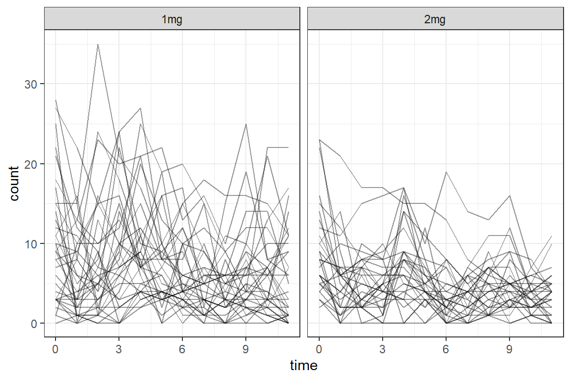

df_long %>% 
  ggplot(aes(x = time, 
             y = count)) +
  geom_smooth(aes(group = id),
              method = "lm",
              color = "gray",
              se = FALSE) +
  facet_grid(. ~ group) + 
  theme_bw()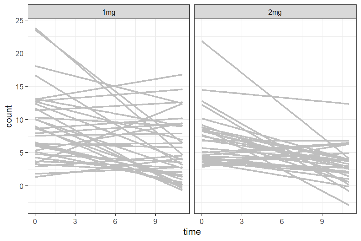

df_long %>% 
  ggplot(aes(x = time, 
             y = count)) +
  geom_smooth(aes(group = id),
              method = "lm",
              formula = y ~ poly(x, 2),
              color = "gray",
              se = FALSE) +
  facet_grid(. ~ group) + 
  theme_bw()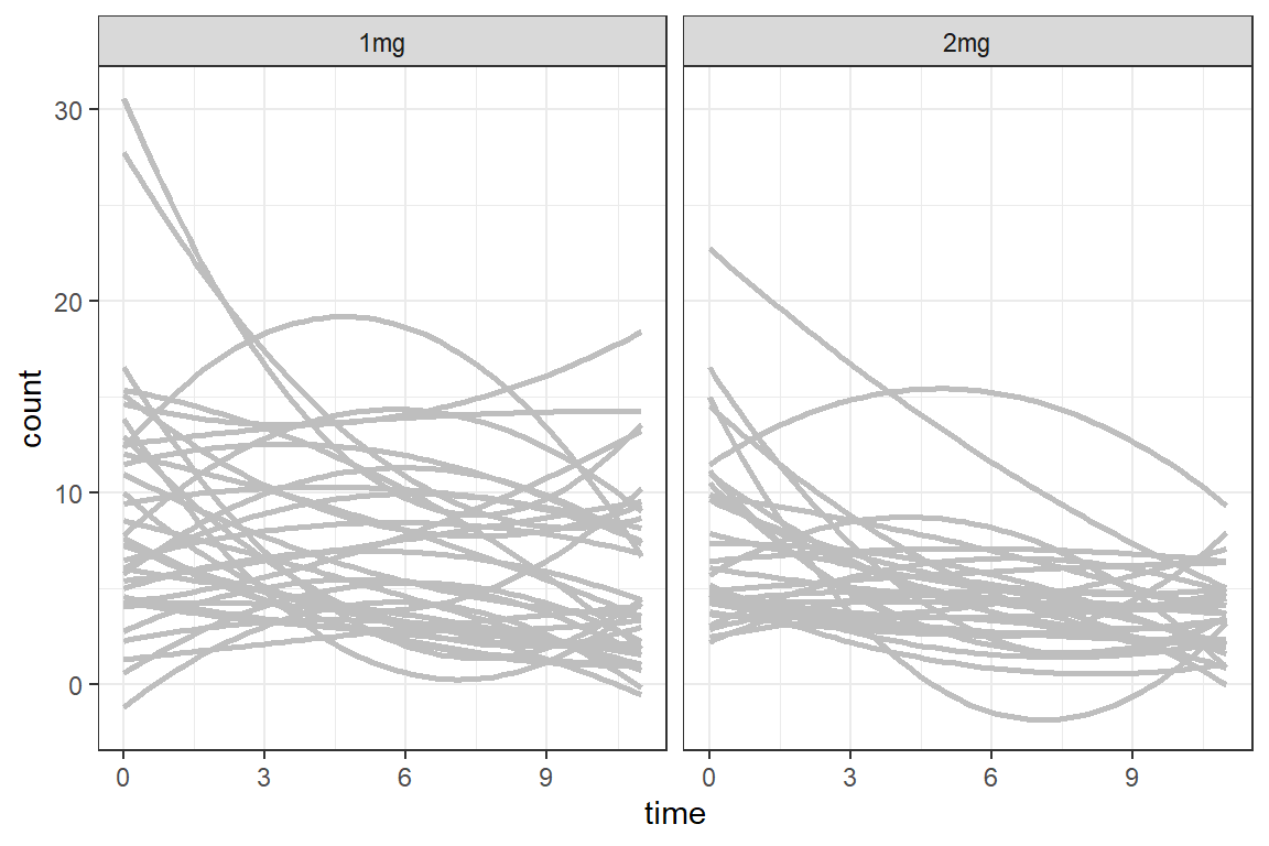

df_long %>% 
  ggplot(aes(x = time, 
             y = count)) +
  geom_line(aes(group = id)) +
  geom_smooth(method = "loess",
              color = "blue",
              se = FALSE) +
  geom_smooth(method = "lm",
              color = "red",
              se = FALSE) +
  facet_grid(. ~ group) + 
  theme_bw()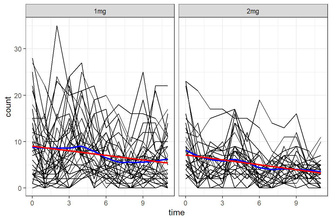

df_long %>% 
  ggplot(aes(x = time, 
             y = log(count + .1))) +
  geom_line(aes(group = id)) +
  geom_smooth(method = "loess",
              color = "blue",
              se = FALSE) +
  geom_smooth(method = "lm",
              color = "red",
              se = FALSE) +
  facet_grid(. ~ group) + 
  theme_bw()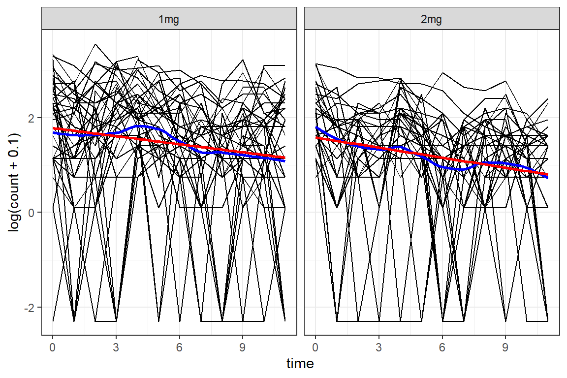

df_long %>% 
  ggplot(aes(x = time, 
             y = count)) +
  geom_smooth(aes(color = "1. Loess"),
              method = "loess",
              se = FALSE) +
  geom_smooth(aes(color = "2. Linear"),
              method = "lm",
              se = FALSE) +
  geom_smooth(aes(color = "3. Quadratic"),
              method = "lm",
              formula = y ~ poly(x, 2),
              se = FALSE) +
  geom_smooth(aes(color = "4. Cubic"),
              method = "lm",
              formula = y ~ poly(x, 3),
              se = FALSE) +
  facet_grid(. ~ group) + 
  theme_bw() +
  labs(color = "Type of Smoother") +
  theme(legend.position = "bottom",
        legend.key.width = unit(1.5, "cm"))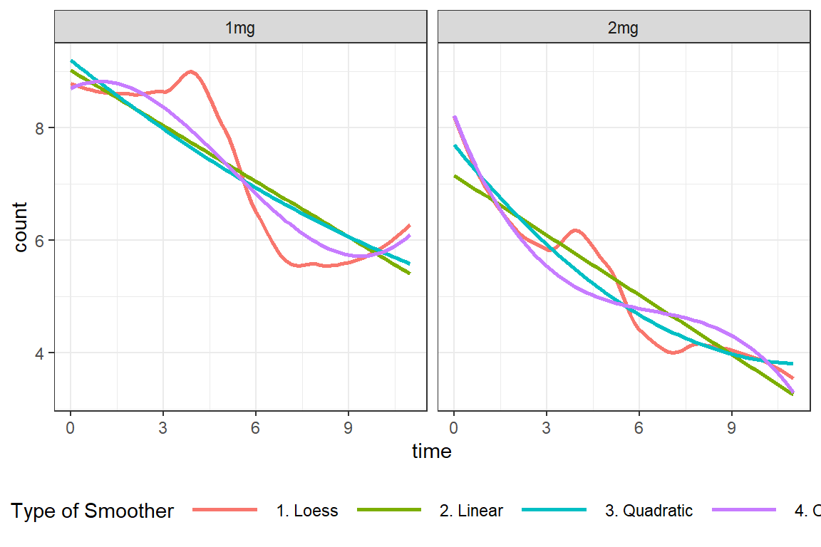

23.3.2.2 Means over Time, BY Group

df_long %>% 
  dplyr::group_by(group, timeF) %>% 
  dplyr::summarise(M = mean(count)) %>% 
  ggplot(aes(x = timeF,
             y = M,
             group = group,
             color = group)) +
  geom_point() + 
  geom_line() + 
  theme_bw() + 
  labs(x = "Four-week Intervals",
       y = "Sample Mean Count",
       color = "Dose")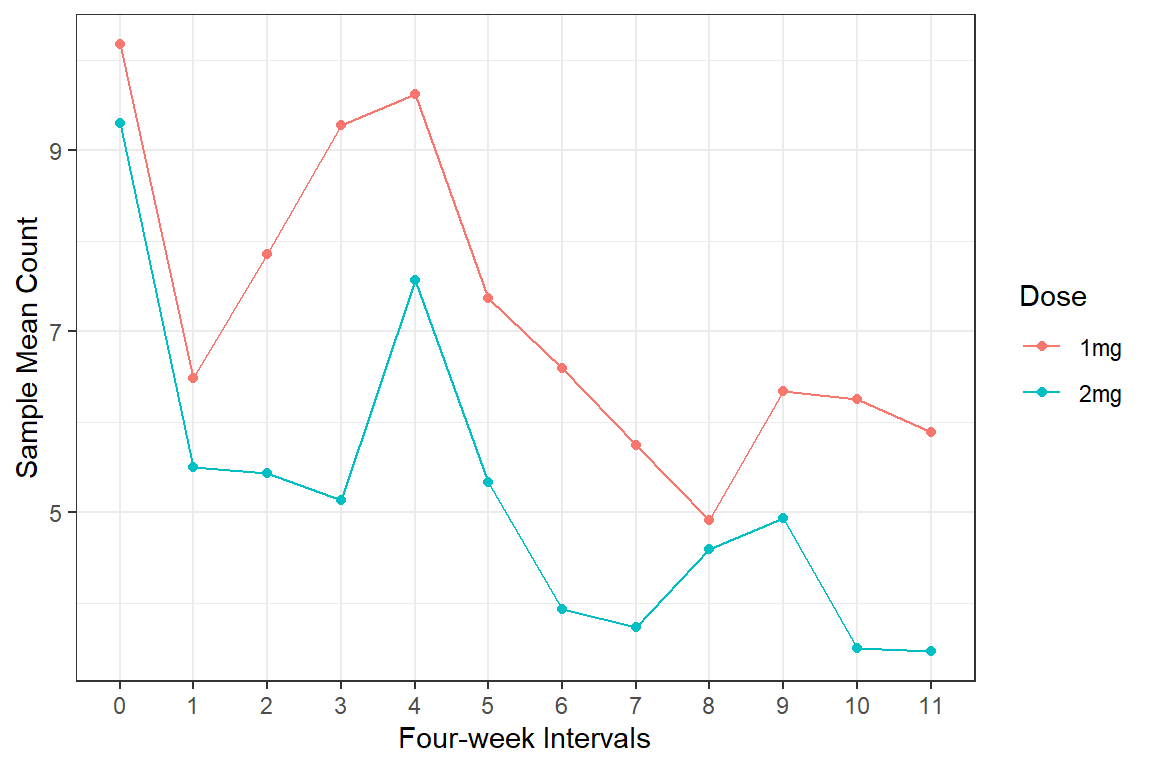

df_long %>% 
  dplyr::group_by(group, timeF) %>% 
  dplyr::summarise(M = mean(log(count + .1))) %>% 
  ggplot(aes(x = timeF,
             y = M,
             group = group,
             color = group)) +
  geom_point() + 
  geom_line() + 
  theme_bw() + 
  labs(x = "Four-week Intervals",
       y = "Sample Mean Count",
       color = "Dose")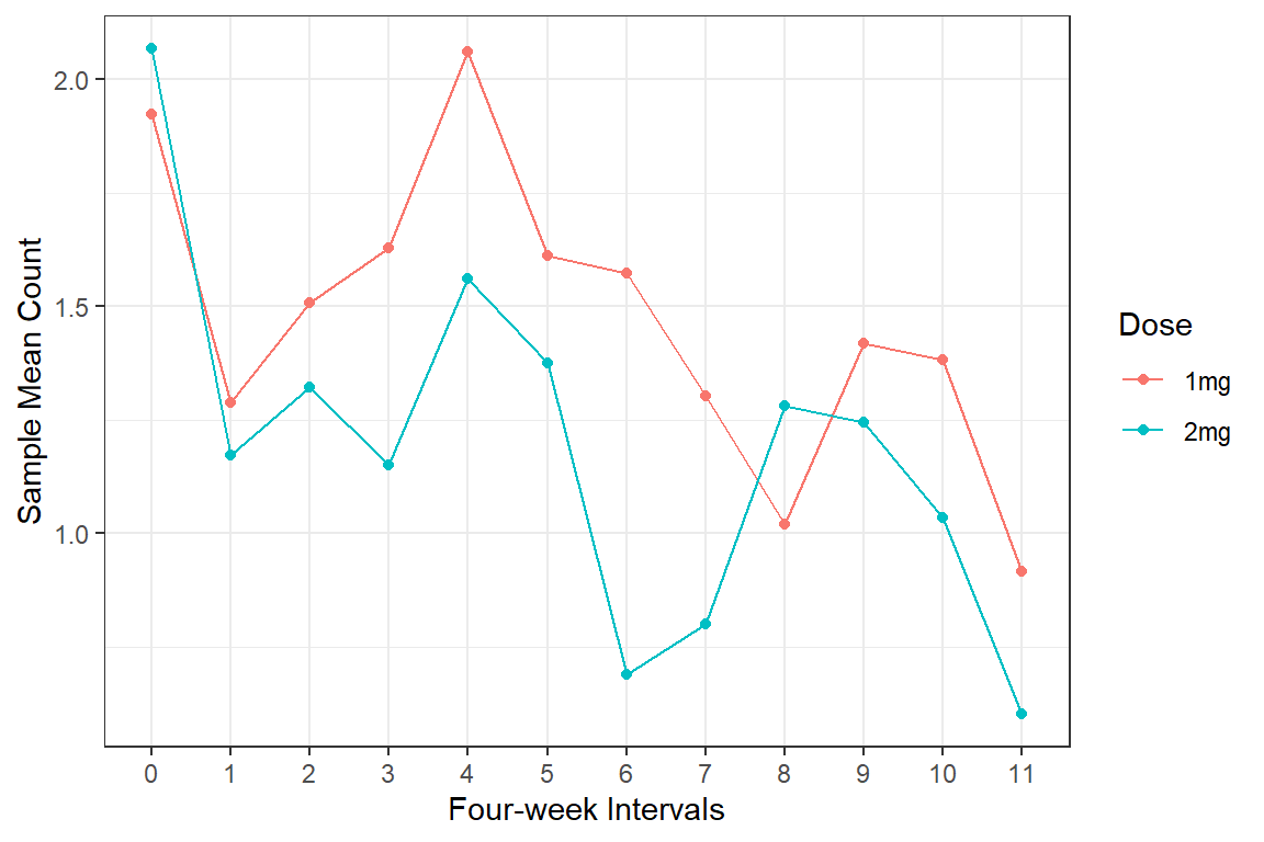

23.4 GEE Analysis

23.4.1 Fit Various Correlation Structures

mod_gee_ex <- geepack::geeglm(count ~ group + time + I(time^2),
                              id = id,
                              data = df_long,
                              family = poisson(link = "log"),
                              corstr = 'exchangeable')

mod_gee_ar <- geepack::geeglm(count ~ group + time + I(time^2),
                              id = id,
                              data = df_long,
                              family = poisson(link = "log"),
                              corstr = "ar1")   

mod_gee_un <- geepack::geeglm(count ~ group + time + I(time^2),
                              id = id,
                              data = df_long,
                              family = poisson(link = "log"),
                              corstr = "unstructured")

23.4.2 Compare Corelation Structures

23.4.2.1 QIC: Model Fit

MuMIn::model.sel(mod_gee_ex, 
                 mod_gee_ar, 
                 mod_gee_un, 
                 rank = "QIC")    #sorts the best to the TOP, uses QIC(I) to choose corelation structure

Model selection table 
           (Intrc) group    time    time^2 corstr qLik   QIC delta weight
mod_gee_ex    2.26     + -0.0714  1.60e-03 exchng 4257 -8491  0.00  0.583
mod_gee_ar    2.39     + -0.1307  6.20e-03    ar1 4247 -8490  1.05  0.346
mod_gee_un    2.14     + -0.0646 -8.25e-06 unstrc 4202 -8487  4.22  0.071
Abbreviations:
 corstr: exchng = 'exchangeable', unstrc = 'unstructured'
Models ranked by QIC(x)

performance::compare_performance(mod_gee_ex, 
                                 mod_gee_ar, 
                                 mod_gee_un,
                                 rank = TRUE)

# Comparison of Model Performance Indices

Name       |  Model |  RMSE | Sigma | Score_log | Score_spherical | AIC weights
-------------------------------------------------------------------------------
mod_gee_ex | geeglm | 5.207 | 2.017 |    -3.617 |           0.028 |       1.000
mod_gee_ar | geeglm | 5.227 | 2.025 |    -3.630 |           0.028 |    6.36e-05
mod_gee_un | geeglm | 5.283 | 2.210 |    -3.687 |           0.028 |    2.16e-24

Name       | AICc weights | BIC weights | Performance-Score
-----------------------------------------------------------
mod_gee_ex |        1.000 |       1.000 |            88.02%
mod_gee_ar |     6.36e-05 |    6.36e-05 |            35.84%
mod_gee_un |     2.16e-24 |    2.16e-24 |            14.29%

23.4.2.2 Model Parameter Table

apaSupp::tab_gees(list("Exchangable"    = mod_gee_ex,
                       "AutoRegressive" = mod_gee_ar,
                       "Unstructured"   = mod_gee_un),
                  narrow = TRUE,
                  caption = "GEE: Main Effects Only, with Quadratic Time")

**Table 23.3**
GEE: Main Effects Only, with Quadratic Time
	Exchangable		AutoRegressive		Unstructured
	IRR	95% CI	IRR	95% CI	IRR	95% CI
(Intercept)	9.61	[7.74, 11.94]***	10.88	[8.81, 13.43]***	8.47	[6.67, 10.74]***
group
1mg	—	—	—	—	—	—
2mg	0.76	[0.59, 0.98]*	0.76	[0.60, 0.98]*	0.77	[0.58, 1.02]
time	0.93	[0.88, 0.99]*	0.88	[0.82, 0.94]***	0.94	[0.87, 1.01]
I(time^2)	1.00	[1.00, 1.01]	1.01	[1.00, 1.01]*	1.00	[0.99, 1.01]
Note.
* p < .05. p < .01. * p < .001.

23.4.3 Add Interaction Terms

mod_gee_ex2 <- geepack::geeglm(count ~ group + time,
                               id = id,
                               data = df_long,
                               family = poisson(link = "log"),
                               corstr = "exchangeable")


mod_gee_ex3 <- geepack::geeglm(count ~ group*time + group*I(time^2),
                               id = id,
                               data = df_long,
                               family = poisson(link = "log"),
                               corstr = "exchangeable")

MuMIn::QIC(mod_gee_ex, 
           mod_gee_ex2,
           mod_gee_ex3, 
           typeR = TRUE)    # NOT the default

              QIC
mod_gee_ex  -8488
mod_gee_ex2 -8488
mod_gee_ex3 -8496

apaSupp::tab_gees(list("Quadratic" = mod_gee_ex,
                       "Linear" = mod_gee_ex2,
                       "Interaction" = mod_gee_ex3),
                  narrow = TRUE,
                  caption = "GEE: Exchangeable")

**Table 23.4**
GEE: Exchangeable
	Quadratic		Linear		Interaction
	IRR	95% CI	IRR	95% CI	IRR	95% CI
(Intercept)	9.61	[7.74, 11.94]***	9.38	[7.73, 11.37]***	9.22	[7.20, 11.79]***
group
1mg	—	—	—	—	—	—
2mg	0.76	[0.59, 0.98]*	0.76	[0.59, 0.98]*	0.84	[0.60, 1.18]
time	0.93	[0.88, 0.99]*	0.95	[0.93, 0.97]***	0.95	[0.88, 1.03]
I(time^2)	1.00	[1.00, 1.01]			1.00	[0.99, 1.01]
group * time
2mg * time					0.95	[0.84, 1.06]
group * I(time^2)
2mg * I(time^2)					1.00	[0.99, 1.01]
Note.
* p < .05. p < .01. * p < .001.

23.4.4 Visualize Best Model

23.4.4.1 Model Parameter Table

apaSupp::tab_gee(mod_gee_ex2)

**Table 23.5**
Parameter Estimates for GEE
	Incident Rate Ratio		Log Scale
	IRR	95% CI	b	(SE)	p
(Intercept)	9.38	[7.73, 11.37]	2.24	(0.10)	< .001***
group
1mg	—	—	—	—
2mg	0.76	[0.59, 0.98]	-0.28	(0.13)	.037*
time	0.95	[0.93, 0.97]	-0.05	(0.01)	< .001***
Note. N = 780 observations on 65 participants. Correlation structure: exchangeable
* p < .05. p < .01. * p < .001.

23.4.4.2 Predict over a Grid

Estimated Marginal Mean Counts

mod_gee_ex2 %>% 
  emmeans::emmeans(pairwise ~group|time,
                   at = list(time = c(0, 5, 10)),
                   type = "response")

$emmeans
time =  0:
 group rate    SE  df lower.CL upper.CL
 1mg   9.38 0.925 777     7.72    11.38
 2mg   7.12 0.729 777     5.82     8.70

time =  5:
 group rate    SE  df lower.CL upper.CL
 1mg   7.14 0.675 777     5.93     8.59
 2mg   5.42 0.497 777     4.52     6.49

time = 10:
 group rate    SE  df lower.CL upper.CL
 1mg   5.43 0.624 777     4.34     6.80
 2mg   4.12 0.440 777     3.34     5.08

Covariance estimate used: vbeta 
Confidence level used: 0.95 
Intervals are back-transformed from the log scale 

$contrasts
time = 0:
 contrast  ratio    SE  df null t.ratio p.value
 1mg / 2mg  1.32 0.174 777    1   2.085  0.0374

time = 5:
 contrast  ratio    SE  df null t.ratio p.value
 1mg / 2mg  1.32 0.174 777    1   2.085  0.0374

time = 10:
 contrast  ratio    SE  df null t.ratio p.value
 1mg / 2mg  1.32 0.174 777    1   2.085  0.0374

Tests are performed on the log scale

23.4.4.3 Plot Estimated Marginal Means

interactions::interact_plot(model = mod_gee_ex2,
                            pred = time,
                            modx = group) # Can NOT do interval ribbons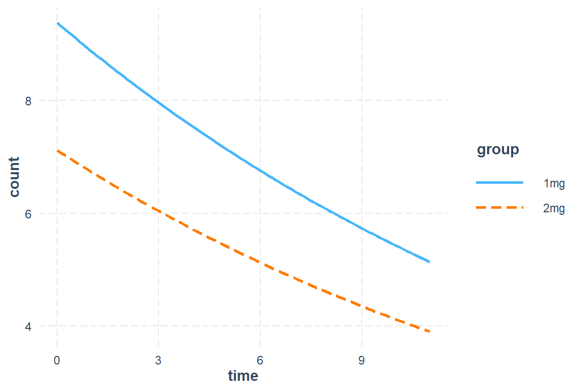

mod_gee_ex2 %>% 
  emmeans::emmeans(~group|time,
                   at = list(time = seq(from = 0, to = 11, by = .1)),
                   type = "response",
                   level = .685) %>% 
  data.frame() %>% 
  ggplot(aes(x = time,
             y = rate,
             group = group)) +
  geom_ribbon(aes(ymin = lower.CL,
                  ymax = upper.CL,
                  fill = group),
              alpha = .2) +
  geom_line(aes(color = group,
                linetype = group)) + 
  theme_bw() + 
  labs(x = "Four-Hour Intervals",
       y = "Estimated Rate\nof Doses per 4 Hour Window",
       color = "Dose",
       fill = "Dose",
       linetype = "Dose") + 
  scale_x_continuous(breaks = seq(from = 0, to = 12, by = 2)) +
  theme(legend.position = "inside",
        legend.position.inside = c(1, 1),
        legend.justification = c(1.1, 1.1),
        legend.background = element_rect(color = "black"),
        legend.key.width = unit(1.5, "cm"))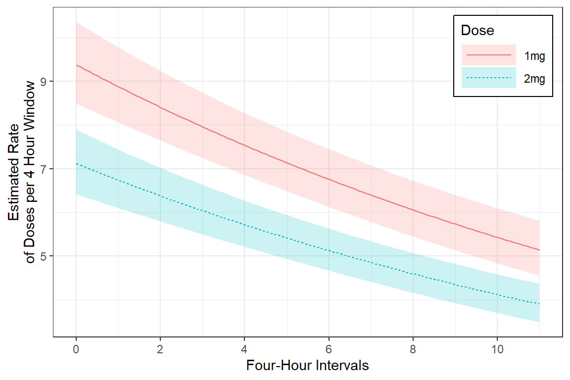

23.5 GLMM Analysis

23.5.1 RI: Random Intercepts Only

mod_glmer_ri <- lme4::glmer(count ~ group + I(time/4) + I((time/4)^2) + (1|id),
                            data = df_long,
                            family = poisson(link = "log"))

summary(mod_glmer_ri)

Generalized linear mixed model fit by maximum likelihood (Laplace
  Approximation) [glmerMod]
 Family: poisson  ( log )
Formula: count ~ group + I(time/4) + I((time/4)^2) + (1 | id)
   Data: df_long

      AIC       BIC    logLik -2*log(L)  df.resid 
     4615      4638     -2303      4605       775 

Scaled residuals: 
   Min     1Q Median     3Q    Max 
-3.505 -1.103 -0.174  0.825  8.581 

Random effects:
 Groups Name        Variance Std.Dev.
 id     (Intercept) 0.246    0.496   
Number of obs: 780, groups:  id, 65

Fixed effects:
              Estimate Std. Error z value Pr(>|z|)    
(Intercept)     2.1347     0.0912   23.40  < 2e-16 ***
group2mg       -0.2713     0.1276   -2.13    0.034 *  
I(time/4)      -0.2855     0.0593   -4.81  1.5e-06 ***
I((time/4)^2)   0.0256     0.0217    1.18    0.238    
---
Signif. codes:  0 '***' 0.001 '**' 0.01 '*' 0.05 '.' 0.1 ' ' 1

Correlation of Fixed Effects:
            (Intr) grp2mg I(t/4)
group2mg    -0.641              
I(time/4)   -0.284  0.000       
I((tm/4)^2)  0.231  0.000 -0.960

23.5.2 RIAS: Random Intercepts and Slopes

mod_glmer_rias <- lme4::glmer(count ~ group + I(time/4) + I((time/4)^2) + 
                                (I(time/4)|id),
                              data = df_long,
                              family = poisson(link = "log"))

summary(mod_glmer_rias)

Generalized linear mixed model fit by maximum likelihood (Laplace
  Approximation) [glmerMod]
 Family: poisson  ( log )
Formula: count ~ group + I(time/4) + I((time/4)^2) + (I(time/4) | id)
   Data: df_long

      AIC       BIC    logLik -2*log(L)  df.resid 
     4440      4473     -2213      4426       773 

Scaled residuals: 
   Min     1Q Median     3Q    Max 
-3.462 -0.965 -0.127  0.758  4.554 

Random effects:
 Groups Name        Variance Std.Dev. Corr 
 id     (Intercept) 0.300    0.548         
        I(time/4)   0.102    0.320    -0.45
Number of obs: 780, groups:  id, 65

Fixed effects:
              Estimate Std. Error z value Pr(>|z|)    
(Intercept)     2.1060     0.0960   21.94   <2e-16 ***
group2mg       -0.2481     0.1274   -1.95   0.0515 .  
I(time/4)      -0.2258     0.0726   -3.11   0.0019 ** 
I((time/4)^2)  -0.0156     0.0222   -0.70   0.4837    
---
Signif. codes:  0 '***' 0.001 '**' 0.01 '*' 0.05 '.' 0.1 ' ' 1

Correlation of Fixed Effects:
            (Intr) grp2mg I(t/4)
group2mg    -0.602              
I(time/4)   -0.412 -0.008       
I((tm/4)^2)  0.226  0.000 -0.792

anova(mod_glmer_ri, mod_glmer_rias)

Data: df_long
Models:
mod_glmer_ri: count ~ group + I(time/4) + I((time/4)^2) + (1 | id)
mod_glmer_rias: count ~ group + I(time/4) + I((time/4)^2) + (I(time/4) | id)
               npar  AIC  BIC logLik -2*log(L) Chisq Df Pr(>Chisq)    
mod_glmer_ri      5 4615 4638  -2303      4605                        
mod_glmer_rias    7 4440 4473  -2213      4426   179  2     <2e-16 ***
---
Signif. codes:  0 '***' 0.001 '**' 0.01 '*' 0.05 '.' 0.1 ' ' 1

apaSupp::tab_glmers(list("RI"   = mod_glmer_ri, 
                        "RIAS" = mod_glmer_rias),
                    caption = "GLMM: Main Effects Models")

**Table 23.6**
GLMM: Main Effects Models
	RI			RIAS
Variable	IRR	[95% CI]	p	IRR	[95% CI]	p
(Intercept)	8.45	[7.07, 10.11]	< .001***	8.22	[6.81, 9.92]	< .001***
group
1mg	—	—		—	—
2mg	0.76	[0.59, 0.98]	.034*	0.78	[0.61, 1.00]	.052
I(time/4)	0.75	[0.67, 0.84]	< .001***	0.80	[0.69, 0.92]	.002**
I((time/4)^2)	1.03	[0.98, 1.07]	.238	0.98	[0.94, 1.03]	.484
id.var__(Intercept)	0.25			0.30
id.cov__(Intercept).I(time/4)				-0.08
id.var__I(time/4)				0.10
AIC	4,615.17			4,440.36
BIC	4,638.47			4,472.97
Log-likelihood	-2,302.59			-2,213.18
Note. N = 780. CI = confidence interval.
* p < .05. p < .01. * p < .001.

23.5.3 RAIS: Add Interaction

See the GLMM - Optimizers page for more information on convergence problems.

mod_glmer_rias2 <- lme4::glmer(count ~ group*I(time/4) + group*I((time/4)^2) + 
                                 ( I(time/4)|id ),
                               data = df_long,
                               control = glmerControl(optimizer ="Nelder_Mead"), 
                               family = poisson(link = "log"))

anova(mod_glmer_rias, mod_glmer_rias2)

Data: df_long
Models:
mod_glmer_rias: count ~ group + I(time/4) + I((time/4)^2) + (I(time/4) | id)
mod_glmer_rias2: count ~ group * I(time/4) + group * I((time/4)^2) + (I(time/4) | id)
                npar  AIC  BIC logLik -2*log(L) Chisq Df Pr(>Chisq)
mod_glmer_rias     7 4440 4473  -2213      4426                    
mod_glmer_rias2    9 4442 4484  -2212      4424  1.93  2       0.38

apaSupp::tab_glmers(list("Main Effects" = mod_glmer_rias,
                         "interactions" = mod_glmer_rias2),
                    caption = "GLMM: Main Effects vs. Interaction")

**Table 23.7**
GLMM: Main Effects vs. Interaction
	Main Effects			interactions
Variable	IRR	[95% CI]	p	IRR	[95% CI]	p
(Intercept)	8.22	[6.81, 9.92]	< .001***	7.84	[6.40, 9.60]	< .001***
group
1mg	—	—		—	—
2mg	0.78	[0.61, 1.00]	.052	0.87	[0.64, 1.18]	.366
I(time/4)	0.80	[0.69, 0.92]	.002**	0.87	[0.72, 1.04]	.133
I((time/4)^2)	0.98	[0.94, 1.03]	.484	0.97	[0.91, 1.02]	.211
group * I(time/4)
2mg * I(time/4)				0.81	[0.61, 1.09]	.162
group * I((time/4)^2)
2mg * I((time/4)^2)				1.05	[0.96, 1.15]	.253
id.var__(Intercept)	0.30			0.30
id.cov__(Intercept).I(time/4)	-0.08			-0.08
id.var__I(time/4)	0.10			0.10
AIC	4,440.36			4,442.42
BIC	4,472.97			4,484.36
Log-likelihood	-2,213.18			-2,212.21
Note. N = 780. CI = confidence interval.
* p < .05. p < .01. * p < .001.

23.5.4 RIAS: Simplify

mod_glmer_rias3 <- lme4::glmer(count ~ group + I(time/4)  + 
                                 ( I(time/4)|id ),
                               data = df_long,
                               control = glmerControl(optimizer ="Nelder_Mead"), 
                               family = poisson(link = "log"))

anova(mod_glmer_rias, mod_glmer_rias3)

Data: df_long
Models:
mod_glmer_rias3: count ~ group + I(time/4) + (I(time/4) | id)
mod_glmer_rias: count ~ group + I(time/4) + I((time/4)^2) + (I(time/4) | id)
                npar  AIC  BIC logLik -2*log(L) Chisq Df Pr(>Chisq)
mod_glmer_rias3    6 4439 4467  -2213      4427                    
mod_glmer_rias     7 4440 4473  -2213      4426  0.49  1       0.48

apaSupp::tab_glmers(list("Quadratic" = mod_glmer_rias,
                         "Linear" = mod_glmer_rias3),
                    caption = "GLMM: Nature of Time")

**Table 23.8**
GLMM: Nature of Time
	Quadratic			Linear
Variable	IRR	[95% CI]	p	IRR	[95% CI]	p
(Intercept)	8.22	[6.81, 9.92]	< .001***	8.34	[6.95, 10.01]	< .001***
group
1mg	—	—		—	—
2mg	0.78	[0.61, 1.00]	.052	0.78	[0.61, 1.00]	.051
I(time/4)	0.80	[0.69, 0.92]	.002**	0.77	[0.70, 0.84]	< .001***
I((time/4)^2)	0.98	[0.94, 1.03]	.484
id.var__(Intercept)	0.30			0.30
id.cov__(Intercept).I(time/4)	-0.08			-0.08
id.var__I(time/4)	0.10			0.10
AIC	4,440.36			4,438.85
BIC	4,472.97			4,466.80
Log-likelihood	-2,213.18			-2,213.42
Note. N = 780. CI = confidence interval.
* p < .05. p < .01. * p < .001.

23.5.5 Visualize Best Model

23.5.5.1 Model Parameter Table

apaSupp::tab_glmer(mod_glmer_rias3)

**Table 23.9**
Parameter Estimates for Generalized Mixed Effects Regression
	Incident Rate Ratio		Log Scale
Variable	IRR	[95% CI]	b	(SE)	p
(Intercept)	8.34	[6.95, 10.01]
group
1mg	—	—	—	—
2mg	0.78	[0.61, 1.00]	-0.25	(0.13)	.051
I(time/4)	0.77	[0.70, 0.84]	-0.27	(0.04)	< .001***
id.var__(Intercept)			0.30
id.cov__(Intercept).I(time/4)			-0.08
id.var__I(time/4)			0.10
Note. p = significance from Wald t-test for parameter estimate using Satterthwaite's method for degrees of freedom.
* p < .05. p < .01. * p < .001.

23.5.5.2 Estimated Marginal Means

mod_glmer_rias3 %>% 
  emmeans::emmeans(pairwise ~group|time,
                   at = list(time = c(0, 5, 10)),
                   type = "response")

$emmeans
time =  0:
 group rate    SE  df asymp.LCL asymp.UCL
 1mg   8.34 0.778 Inf      6.95     10.01
 2mg   6.51 0.658 Inf      5.34      7.93

time =  5:
 group rate    SE  df asymp.LCL asymp.UCL
 1mg   5.98 0.526 Inf      5.03      7.11
 2mg   4.67 0.445 Inf      3.87      5.62

time = 10:
 group rate    SE  df asymp.LCL asymp.UCL
 1mg   4.29 0.485 Inf      3.44      5.35
 2mg   3.35 0.395 Inf      2.65      4.22

Confidence level used: 0.95 
Intervals are back-transformed from the log scale 

$contrasts
time = 0:
 contrast  ratio    SE  df null z.ratio p.value
 1mg / 2mg  1.28 0.163 Inf    1   1.948  0.0514

time = 5:
 contrast  ratio    SE  df null z.ratio p.value
 1mg / 2mg  1.28 0.163 Inf    1   1.948  0.0514

time = 10:
 contrast  ratio    SE  df null z.ratio p.value
 1mg / 2mg  1.28 0.163 Inf    1   1.948  0.0514

Tests are performed on the log scale

23.5.5.3 Plot Estimated Marginal Means

interactions::interact_plot(model = mod_glmer_rias3,
                            pred = time,
                            modx = group,
                            interval = TRUE,
                            int.width = .685)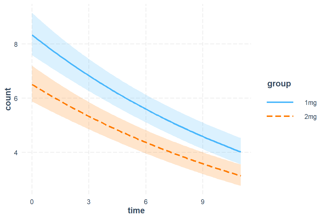

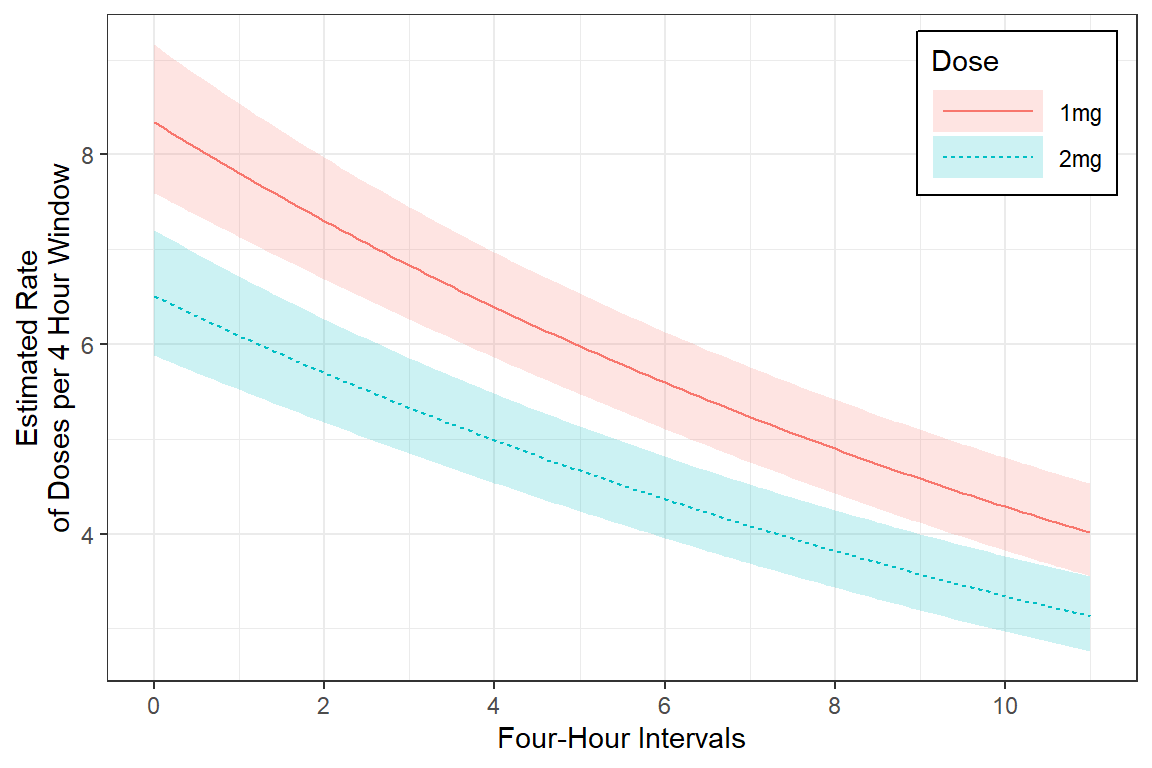
mod_glmer_rias3 %>% 
  emmeans::emmeans(~group|time,
                   at = list(time = seq(from = 0, to = 11, by = .1)),
                   type = "response",
                   level = .685) %>% 
  data.frame() %>% 
  ggplot(aes(x = time,
             y = rate,
             group = group)) +
  geom_ribbon(aes(ymin = asymp.LCL,
                  ymax = asymp.UCL,
                  fill = group),
              alpha = .2) +
  geom_line(aes(color = group,
                linetype = group)) + 
  theme_bw() + 
  labs(x = "Four-Hour Intervals",
       y = "Estimated Rate\nof Doses per 4 Hour Window",
       color = "Dose",
       fill = "Dose",
       linetype = "Dose") + 
  scale_x_continuous(breaks = seq(from = 0, to = 12, by = 2)) +
  theme(legend.position = "inside",
        legend.position.inside = c(1, 1),
        legend.justification = c(1.1, 1.1),
        legend.background = element_rect(color = "black"),
        legend.key.width = unit(1.5, "cm"))