18 GEE, Count Outcome: Antibiotics for Leprosy

18.1 PREPARATION

18.1.1 Load Packages

install.packages("devtools")
devtools::install_github("sarbearschwartz/apaSupp") # updated 10/14/2025

Load/activate these packages

library(tidyverse)    
library(flextable)
library(apaSupp)      # Not on CRAN, on GitHub (see above)
library(psych) 
library(lme4)         
library(lmerTest)
library(corrplot)      
library(geepack)       
library(MuMIn)  
library(interactions)
library(performance)      

library(HSAUR)        # package with the dataset

18.1.2 Background

The following example is presented in the textbook: “Applied Longitudinal Analysis” by Garrett Fitzmaurice, Nan Laird & James Ware

The dataset maybe downloaded from: https://content.sph.harvard.edu/fitzmaur/ala/

Data on count of leprosy bacilli pre- and post-treatment from a clinical trial of antibiotics for leprosy.

Source: Table 14.2.1 (page 422) in Snedecor, G.W. and Cochran, W.G. (1967). Statistical Methods, (6th edn). Ames, Iowa: Iowa State University Press

With permission of Iowa State University Press.

Reference: Snedecor, G.W. and Cochran, W.G. (1967). Statistical Methods, (6th edn). Ames, Iowa: Iowa State University Press

The Background

The dataset consists of count data from a placebo-controlled clinical trial of 30 patients with leprosy at the Eversley Childs Sanitorium in the Philippines. Participants in the study were randomized to either of two antibiotics (denoted treatment drug A and B) or to a placebo (denoted treatment drug C).

Prior to receiving treatment, baseline data on the number of leprosy bacilli at six sites of the body where the bacilli tend to congregate were recorded for each patient. After several months of treatment, the number of leprosy bacilli at six sites of the body were recorded a second time. The outcome variable is the total count of the number of leprosy bacilli at the six sites.

The Research Question

In this study, the question of main scientific interest is whether treatment with antibiotics (drugs A and B) reduces the abundance of leprosy bacilli at the six sites of the body when compared to placebo (drug C).

The Data

Outcome or dependent variable(s)
- count.pre Pre-Treatment Bacilli Count
- count.post Post-Treatment Bacilli Count
Main predictor or independent variable of interest
- drug the treatment group: antibiotics (drugs A and B) or placebo (drug C)

18.1.3 Enter the data by hand!

df_raw <- tibble::tribble(
  ~drug, ~count_pre, ~count_post,
  "A",      11,     6,    "B",       6,     0,    "C",      16,    13,
  "A",       8,     0,    "B",       6,     2,    "C",      13,    10,
  "A",       5,     2,    "B",       7,     3,    "C",      11,    18,
  "A",      14,     8,    "B",       8,     1,    "C",       9,     5,
  "A",      19,    11,    "B",      18,    18,    "C",      21,    23,
  "A",       6,     4,    "B",       8,     4,    "C",      16,    12,
  "A",      10,    13,    "B",      19,    14,    "C",      12,     5,
  "A",       6,     1,    "B",       8,     9,    "C",      12,    16,
  "A",      11,     8,    "B",       5,     1,    "C",       7,     1,
  "A",       3,     0,    "B",      15,     9,    "C",      12,    20)

18.1.4 Wide Format

df_wide <- df_raw %>% 
  dplyr::mutate(drug = factor(drug)) %>% 
  dplyr::mutate(id = row_number()) %>% 
  dplyr::select(id, drug, count_pre, count_post)

str(df_wide)

tibble [30 × 4] (S3: tbl_df/tbl/data.frame)
 $ id        : int [1:30] 1 2 3 4 5 6 7 8 9 10 ...
 $ drug      : Factor w/ 3 levels "A","B","C": 1 2 3 1 2 3 1 2 3 1 ...
 $ count_pre : num [1:30] 11 6 16 8 6 13 5 7 11 14 ...
 $ count_post: num [1:30] 6 0 13 0 2 10 2 3 18 8 ...

df_wide %>%
  psych::headTail() %>% 
  flextable::flextable() %>% 
  apaSupp::theme_apa(caption = "Wide format of the Data")

**Table 18.1**
Wide format of the Data
id	drug	count_pre	count_post
1	A	11	6
2	B	6	0
3	C	16	13
4	A	8	0
...		...	...
27	C	7	1
28	A	3	0
29	B	15	9
30	C	12	20

18.1.5 Long Format

df_long <- df_wide %>% 
  tidyr::gather(key = obs,
                value = count,
                starts_with("count")) %>% 
  dplyr::mutate(time = case_when(obs == "count_pre" ~ 0,
                                 obs == "count_post" ~ 1)) %>% 
  dplyr::select(id, drug, time, count) %>% 
  dplyr::arrange(id, time)

str(df_long)

tibble [60 × 4] (S3: tbl_df/tbl/data.frame)
 $ id   : int [1:60] 1 1 2 2 3 3 4 4 5 5 ...
 $ drug : Factor w/ 3 levels "A","B","C": 1 1 2 2 3 3 1 1 2 2 ...
 $ time : num [1:60] 0 1 0 1 0 1 0 1 0 1 ...
 $ count: num [1:60] 11 6 6 0 16 13 8 0 6 2 ...

df_long %>%
  psych::headTail() %>% 
  flextable::flextable() %>% 
  apaSupp::theme_apa(caption = "Long format of the Data")

**Table 18.2**
Long format of the Data
id	drug	time	count
1	A	0	11
1	A	1	6
2	B	0	6
2	B	1	0
...		...	...
29	B	0	15
29	B	1	9
30	C	0	12
30	C	1	20

18.2 Exploratory Data Analysis

18.2.1 Summary Statistics

df_long %>% 
  dplyr::group_by(drug, time) %>% 
  dplyr::summarise(N = n(),
                   M = mean(count),
                   VAR = var(count),
                   SD = sd(count)) %>% 
  flextable::as_grouped_data(groups = "drug") %>% 
  flextable::flextable() %>% 
  apaSupp::theme_apa(caption = "Summary for each group at each time")

**Table 18.3**
Summary for each group at each time
drug	time	N	M	VAR	SD
A
	0.00	10	9.30	22.68	4.76
	1.00	10	5.30	21.57	4.64
B
	0.00	10	10.00	27.56	5.25
	1.00	10	6.10	37.88	6.15
C
	0.00	10	12.90	15.66	3.96
	1.00	10	12.30	51.12	7.15

18.2.2 Visualize

df_long %>% 
  dplyr::mutate(time_name = case_when(time == 0 ~ "Pre",
                                      time == 1 ~ "Post") %>% 
                  factor(levels = c("Pre", "Post"))) %>% 
  dplyr::mutate(drug_name = fct_recode(drug,
                                       "Antibiotic A" = "A",
                                       "Antibiotic B" = "B",
                                       "Placebo" = "C")) %>% 
  ggplot(aes(x = time_name,
             y = count)) +
  geom_line(aes(group = id)) +
  facet_grid(.~ drug_name) +
  theme_bw() +
  labs(x = NULL,
       y = "Number of Leprosy Bacilli at Six Sites of the Body")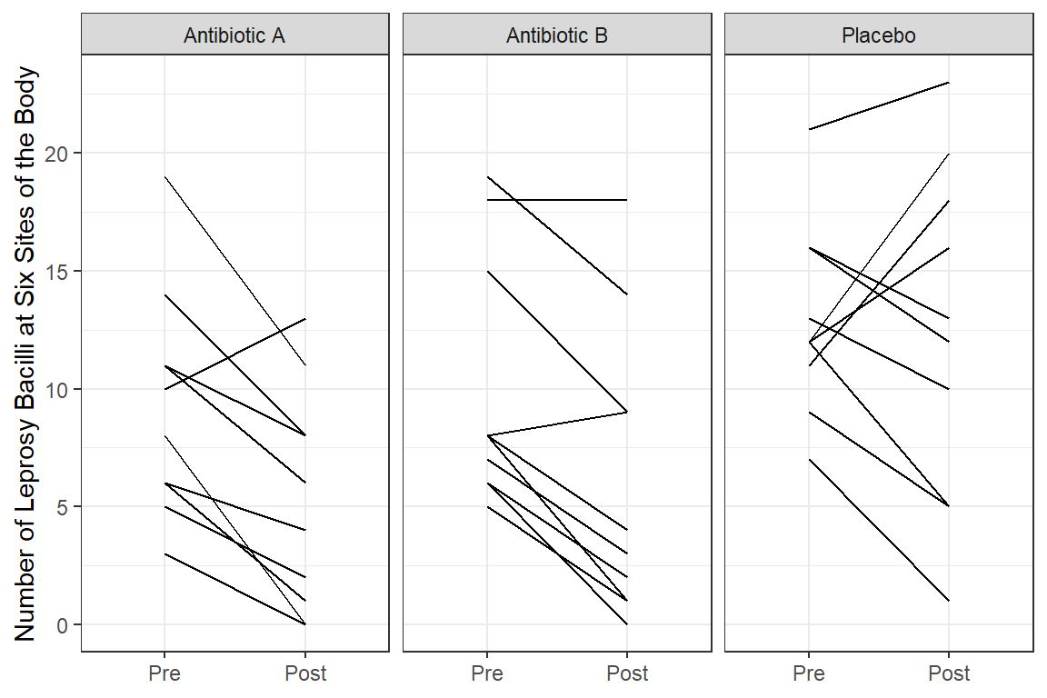

df_long %>% 
  dplyr::mutate(time_name = case_when(time == 0 ~ "Pre",
                                      time == 1 ~ "Post") %>% 
                  factor(levels = c("Pre", "Post"))) %>% 
  dplyr::mutate(drug_name = fct_recode(drug,
                                       "Antibiotic A" = "A",
                                       "Antibiotic B" = "B",
                                       "Placebo" = "C")) %>% 
  ggplot(aes(x = time,
             y = count)) +
  geom_line(aes(group = id),
            color = "gray") +
  geom_smooth(aes(group = drug),
              method = "lm") +
  facet_grid(.~ drug_name) +
  theme_bw() +
  labs(x = NULL,
       y = "Number of Leprosy Bacilli at Six Sites of the Body")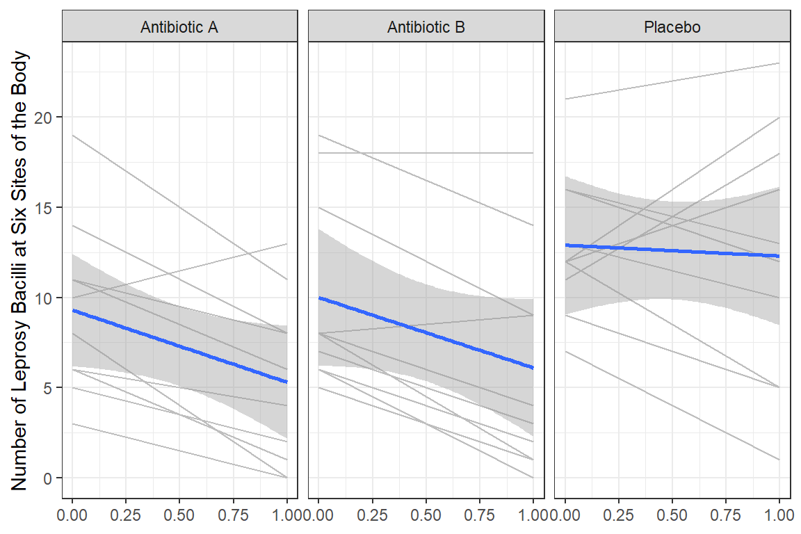

df_long %>% 
  dplyr::mutate(time_name = case_when(time == 0 ~ "Pre",
                                      time == 1 ~ "Post") %>% 
                  factor(levels = c("Pre", "Post"))) %>% 
  dplyr::mutate(drug_name = fct_recode(drug,
                                       "Antibiotic A" = "A",
                                       "Antibiotic B" = "B",
                                       "Placebo" = "C")) %>% 
  ggplot(aes(x = time,
             y = count)) +
  geom_smooth(aes(group = drug,
                  color = drug_name,
                  fill = drug_name),
              method = "lm",
              alpha = .2) +
  theme_bw() +
  labs(x = NULL,
       y = "Number of Leprosy Bacilli at Six Sites of the Body",
       color = NULL,
       fill = NULL) +
  scale_x_continuous(breaks = 0:1,
                     labels = c("Pre-Treatment", "Post-Treatment"))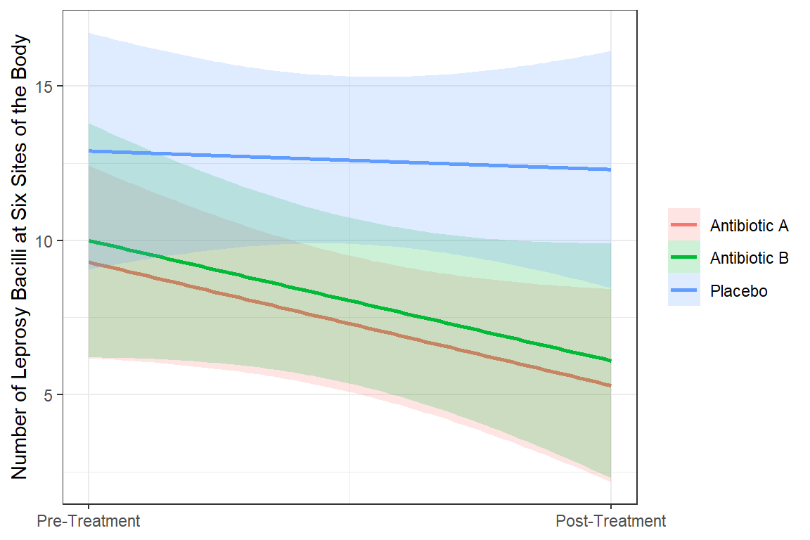

18.3 Generalized Estimating Equations (GEE)

18.3.1 Explore Various Correlation Structures

18.3.1.1 Fit the models - to determine correlation structure

The gee() function in the gee package

mod_geeglm_ind <- geepack::geeglm(count ~ drug*time,
                                  data = df_long,
                                  family = poisson(link = "log"),
                                  id = id,
                                  waves = time,
                                  corstr = "independence")

mod_geeglm_exc <- geepack::geeglm(count ~ drug*time,
                                  data = df_long,
                                  family = poisson(link = "log"),
                                  id = id,
                                  waves = time,
                                  corstr = "exchangeable")

summary(mod_geeglm_ind)


Call:
geepack::geeglm(formula = count ~ drug * time, family = poisson(link = "log"), 
    data = df_long, id = id, waves = time, corstr = "independence")

 Coefficients:
            Estimate Std.err   Wald Pr(>|W|)    
(Intercept)   2.2300  0.1536 210.74   <2e-16 ***
drugB         0.0726  0.2200   0.11   0.7415    
drugC         0.3272  0.1791   3.34   0.0677 .  
time         -0.5623  0.1760  10.21   0.0014 ** 
drugB:time    0.0680  0.2460   0.08   0.7822    
drugC:time    0.5147  0.2206   5.45   0.0196 *  
---
Signif. codes:  0 '***' 0.001 '**' 0.01 '*' 0.05 '.' 0.1 ' ' 1

Correlation structure = independence 
Estimated Scale Parameters:

            Estimate Std.err
(Intercept)     3.13   0.513
Number of clusters:   30  Maximum cluster size: 2

summary(mod_geeglm_exc)


Call:
geepack::geeglm(formula = count ~ drug * time, family = poisson(link = "log"), 
    data = df_long, id = id, waves = time, corstr = "exchangeable")

 Coefficients:
            Estimate Std.err   Wald Pr(>|W|)    
(Intercept)   2.2300  0.1536 210.74   <2e-16 ***
drugB         0.0726  0.2200   0.11   0.7415    
drugC         0.3272  0.1791   3.34   0.0677 .  
time         -0.5623  0.1760  10.21   0.0014 ** 
drugB:time    0.0680  0.2460   0.08   0.7822    
drugC:time    0.5147  0.2206   5.45   0.0196 *  
---
Signif. codes:  0 '***' 0.001 '**' 0.01 '*' 0.05 '.' 0.1 ' ' 1

Correlation structure = exchangeable 
Estimated Scale Parameters:

            Estimate Std.err
(Intercept)     3.13   0.513
  Link = identity 

Estimated Correlation Parameters:
      Estimate Std.err
alpha    0.735   0.081
Number of clusters:   30  Maximum cluster size: 2

18.3.1.2 Parameter Estimates

apaSupp::tab_gees(list("Independence" = mod_geeglm_ind,
                       "Exchangeable" = mod_geeglm_exc),
                  caption = "GEE - Estimates on Count Scale (RR)")

**Table 18.4**
GEE - Estimates on Count Scale (RR)
	Independence			Exchangeable
	IRR	95% CI	p	IRR	95% CI	p
(Intercept)	9.30	[6.88, 12.57]	< .001***	9.30	[6.88, 12.57]	< .001***
drug
A	—	—		—	—
B	1.08	[0.70, 1.65]	.741	1.08	[0.70, 1.65]	.741
C	1.39	[0.98, 1.97]	.068	1.39	[0.98, 1.97]	.068
time	0.57	[0.40, 0.80]	.001**	0.57	[0.40, 0.80]	.001**
drug * time
B * time	1.07	[0.66, 1.73]	.782	1.07	[0.66, 1.73]	.782
C * time	1.67	[1.09, 2.58]	.020*	1.67	[1.09, 2.58]	.020*
Note.
* p < .05. p < .01. * p < .001.

18.3.1.3 Manual Extraction

mod_geeglm_exc %>% coef() %>% exp()

(Intercept)       drugB       drugC        time  drugB:time  drugC:time 
       9.30        1.08        1.39        0.57        1.07        1.67

0.5699*1.6731

[1] 0.953

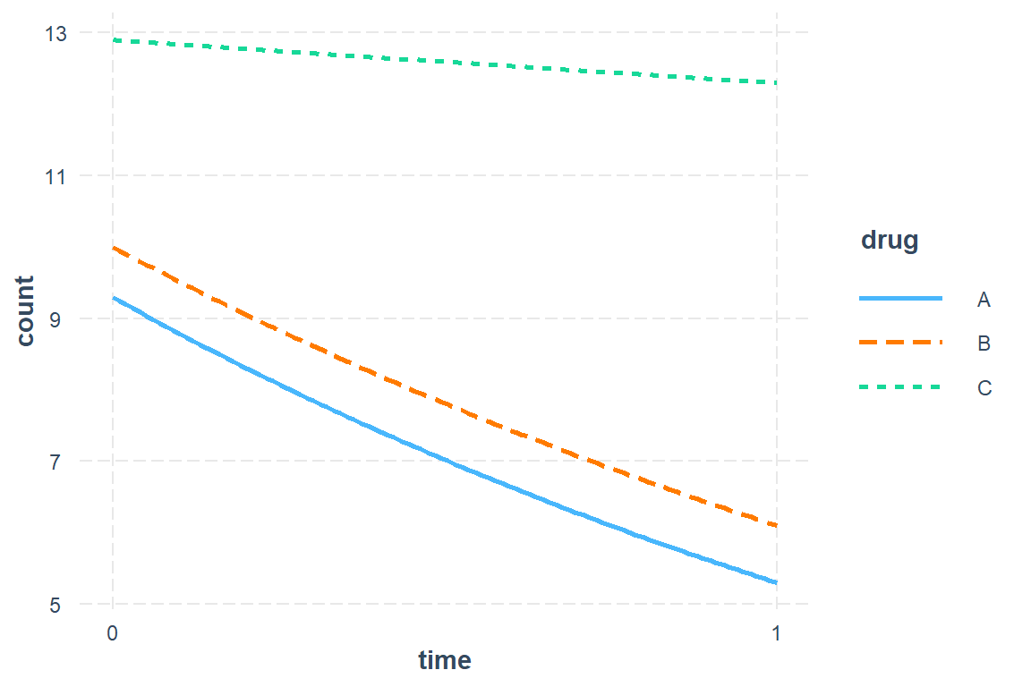
18.3.2 Interpretation

Antibiotic A Group: Starts with mean of 9.3 and drops by 45% (nearly cut in half) over the course of treatment.
Antibiotic B Group: Starts at about the same mean at Antibiotic A group and experiences the same decrease.
Control Group (C): Starts at about the same mean at Antibiotic A group BUT experiences a less than a 5% decrease over the student period while on the placebo pills.

18.3.3 Visualize the Final Model

18.3.3.1 Quick

interactions::interact_plot(model = mod_geeglm_exc,
                            pred = time,
                            modx = drug)

18.3.3.2 More Polished

mod_geeglm_exc %>% 
  emmeans::emmeans(~ drug*time,
                   type = "response")

 drug time rate   SE df lower.CL upper.CL
 A       0  9.3 1.43 54     6.83    12.65
 B       0 10.0 1.58 54     7.29    13.71
 C       0 12.9 1.19 54    10.73    15.51
 A       1  5.3 1.39 54     3.13     8.98
 B       1  6.1 1.85 54     3.32    11.19
 C       1 12.3 2.14 54     8.67    17.45

Covariance estimate used: vbeta 
Confidence level used: 0.95 
Intervals are back-transformed from the log scale

mod_geeglm_exc %>% 
  emmeans::emmeans(~ drug*time,
                   type = "response") %>% 
  data.frame()

  drug time rate   SE df lower.CL upper.CL
1    A    0  9.3 1.43 54     6.83    12.65
2    B    0 10.0 1.57 54     7.29    13.71
3    C    0 12.9 1.19 54    10.73    15.51
4    A    1  5.3 1.39 54     3.13     8.98
5    B    1  6.1 1.85 54     3.32    11.19
6    C    1 12.3 2.14 54     8.67    17.45

mod_geeglm_exc %>% 
  emmeans::emmeans(~ drug*time,
                   type = "response",
                   level = .68) %>% 
  data.frame() %>% 
  dplyr::mutate(time_name = case_when(time == 0 ~ "Pre",
                                      time == 1 ~ "Post") %>% 
                  factor(levels = c("Pre", "Post"))) %>% 
  dplyr::mutate(drug_name = fct_recode(drug,
                                       "Antibiotic A" = "A",
                                       "Antibiotic B" = "B",
                                       "Placebo" = "C")) %>% 
  ggplot(aes(x = time_name,
             y = rate,
             group = drug_name %>% fct_rev,
             color = drug_name %>% fct_rev)) +
  geom_errorbar(aes(ymin = lower.CL,
                    ymax = upper.CL),
                width = .3,
                position = position_dodge(width = .25)) +
  geom_point(position = position_dodge(width = .25)) +
  geom_line(position = position_dodge(width = .25)) +
  theme_bw() +
  labs(x = NULL,
       y = "Estimated Marginal Mean\nNumber of Leprosy Bacilli at Six Sites of the Body",
       color = NULL) +
  theme(legend.position = c(0, 0),
        legend.justification = c(-0.1, -0.1),
        legend.background = element_rect(color = "black"))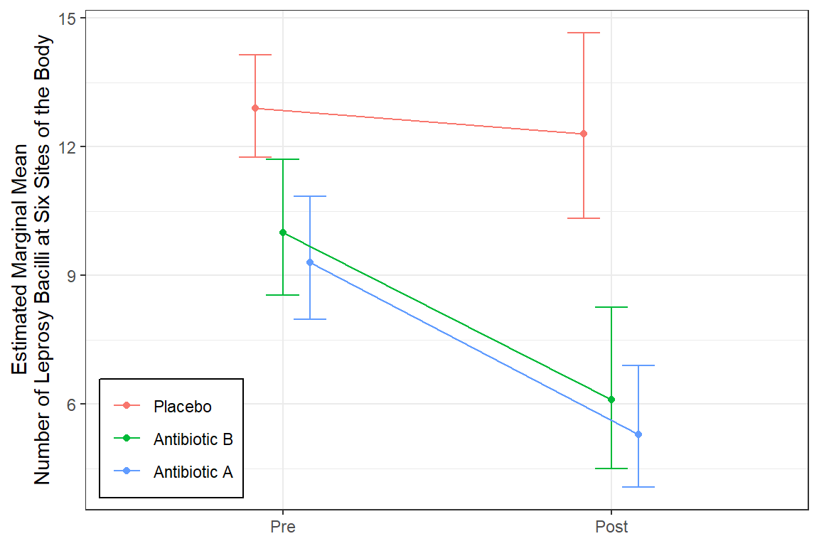

18.4 Follow-up Analysis

18.4.1 Collapse the Predictor

df_remodel <- df_long %>% 
  dplyr::mutate(antibiotic = drug %>% 
                  forcats::fct_collapse(yes = c("A", "B"),
                                        no = c("C")))

18.4.2 Reduce the Model - `gee::gee()`

mod_geeglm_exc2 <- geepack::geeglm(count ~ antibiotic:time ,
                                data = df_remodel,
                                family = poisson(link = "log"),
                                id = id,
                                waves = time,
                                corstr = "exchangeable")

summary(mod_geeglm_exc2)


Call:
geepack::geeglm(formula = count ~ antibiotic:time, family = poisson(link = "log"), 
    data = df_remodel, id = id, waves = time, corstr = "exchangeable")

 Coefficients:
                   Estimate  Std.err Wald Pr(>|W|)    
(Intercept)         2.37335  0.08014  877  < 2e-16 ***
antibioticyes:time -0.53068  0.11306   22  2.7e-06 ***
antibioticno:time  -0.00286  0.15700    0     0.99    
---
Signif. codes:  0 '***' 0.001 '**' 0.01 '*' 0.05 '.' 0.1 ' ' 1

Correlation structure = exchangeable 
Estimated Scale Parameters:

            Estimate Std.err
(Intercept)     3.23    0.52
  Link = identity 

Estimated Correlation Parameters:
      Estimate Std.err
alpha    0.738   0.081
Number of clusters:   30  Maximum cluster size: 2

18.4.3 Compare Parameters

apaSupp::tab_gees(list("Original" = mod_geeglm_exc,
                       "Refit" = mod_geeglm_exc2))

**Table 18.5**
Compare GEE Models
	Original			Refit
	IRR	95% CI	p	IRR	95% CI	p
(Intercept)	9.30	[6.88, 12.57]	< .001***	10.73	[9.17, 12.56]	< .001***
drug
A	—	—
B	1.08	[0.70, 1.65]	.741
C	1.39	[0.98, 1.97]	.068
time	0.57	[0.40, 0.80]	.001**
drug * time
B * time	1.07	[0.66, 1.73]	.782
C * time	1.67	[1.09, 2.58]	.020*
antibiotic * time
yes * time				0.59	[0.47, 0.73]	< .001***
no * time				1.00	[0.73, 1.36]	.985
Note.
* p < .05. p < .01. * p < .001.

18.4.4 Interpretation

The grand mean is a count of 10.73 at pre-treatment.
The mean count dropped by about 40% among those on antibiotics, but there was no decrease for those on placebo pills, exp(b) = 0.592, p < .05, 95% CI [0.476, 0.74].

18.4.5 Visualize

18.4.5.1 Quick

interactions::interact_plot(model = mod_geeglm_exc2,
                            pred = time,
                            modx = antibiotic) +
  theme_bw()

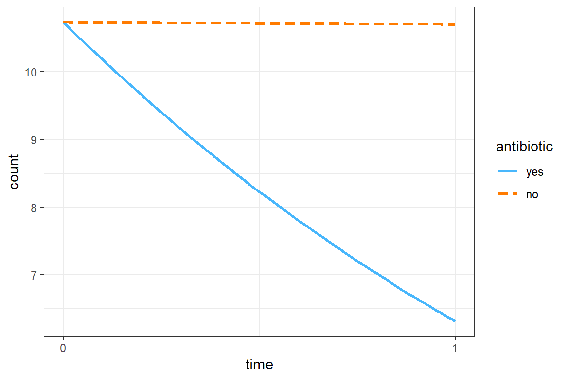
18.4.5.2 More Polished

mod_geeglm_exc2 %>% 
  emmeans::emmeans(~ antibiotic*time,
                   type = "response",
                   level = .68) %>% 
  data.frame() %>% 
  dplyr::mutate(time_name = case_when(time == 0 ~ "Pre",
                                      time == 1 ~ "Post") %>% 
                  factor(levels = c("Pre", "Post"))) %>% 
  ggplot(aes(x = time_name,
             y = rate,
             group = antibiotic,
             color = antibiotic)) +
  geom_errorbar(aes(ymin = lower.CL,
                    ymax = upper.CL),
                width = .3,
                position = position_dodge(width = .25)) +
  geom_point(position = position_dodge(width = .25)) +
  geom_line(position = position_dodge(width = .25)) +
  theme_bw() +
  labs(x = NULL,
       y = "Estimated Marginal Mean\nNumber of Leprosy Bacilli at Six Sites of the Body",
       color = "Antibiotic A or B") +
  theme(legend.position = c(0, 0),
        legend.justification = c(-0.1, -0.1),
        legend.background = element_rect(color = "black"))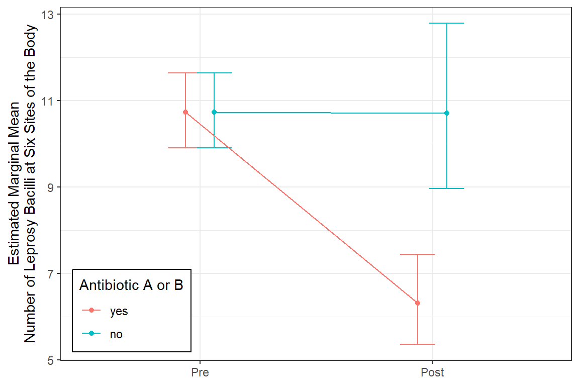

mod_geeglm_exc2 %>% 
  emmeans::emmeans(pairwise ~ time | antibiotic,
                   adjust = "none")

$emmeans
antibiotic = yes:
 time emmean     SE df lower.CL upper.CL
    0   2.37 0.0801 57     2.21     2.53
    1   1.84 0.1640 57     1.51     2.17

antibiotic = no:
 time emmean     SE df lower.CL upper.CL
    0   2.37 0.0801 57     2.21     2.53
    1   2.37 0.1770 57     2.02     2.73

Covariance estimate used: vbeta 
Results are given on the log (not the response) scale. 
Confidence level used: 0.95 

$contrasts
antibiotic = yes:
 contrast      estimate    SE df t.ratio p.value
 time0 - time1    0.531 0.113 57   4.690  <.0001

antibiotic = no:
 contrast      estimate    SE df t.ratio p.value
 time0 - time1    0.003 0.157 57   0.020  0.9860

Results are given on the log (not the response) scale.

mod_geeglm_exc2 %>% 
  emmeans::emmeans(pairwise ~ time | antibiotic,
                   type = "response",
                   adjust = "none")

$emmeans
antibiotic = yes:
 time  rate   SE df lower.CL upper.CL
    0 10.73 0.86 57     9.14    12.60
    1  6.31 1.03 57     4.55     8.76

antibiotic = no:
 time  rate   SE df lower.CL upper.CL
    0 10.73 0.86 57     9.14    12.60
    1 10.70 1.90 57     7.50    15.27

Covariance estimate used: vbeta 
Confidence level used: 0.95 
Intervals are back-transformed from the log scale 

$contrasts
antibiotic = yes:
 contrast      ratio    SE df null t.ratio p.value
 time0 / time1   1.7 0.192 57    1   4.690  <.0001

antibiotic = no:
 contrast      ratio    SE df null t.ratio p.value
 time0 / time1   1.0 0.158 57    1   0.020  0.9860

Tests are performed on the log scale

18.5 Conclusion