6 MLM, 3 levels: Nurse’s Stress Intervention

Download/install a new GitHub package
install.packages("devtools")
devtools::install_github("sarbearschwartz/apaSupp") # updated 9/17/2025
Load/activate these packages
library(haven)
library(tidyverse)
library(flextable)
library(apaSupp)      # Not on CRAN, on GitHub (see above)
library(lme4)
library(lmerTest)
library(optimx)
library(insight)
library(performance)
library(interactions)
library(emmeans)
library(effects)
library(sjPlot)
6.1 Background
The text “Multilevel Analysis: Techniques and Applications, Third Edition” (Hox, Moerbeek, and Van de Schoot 2017) has a companion website which includes links to all the data files used throughout the book (housed on the book’s GitHub repository).
The following example is used through out Hox, Moerbeek, and Van de Schoot (2017)’s chapater 2.
From Appendix E:
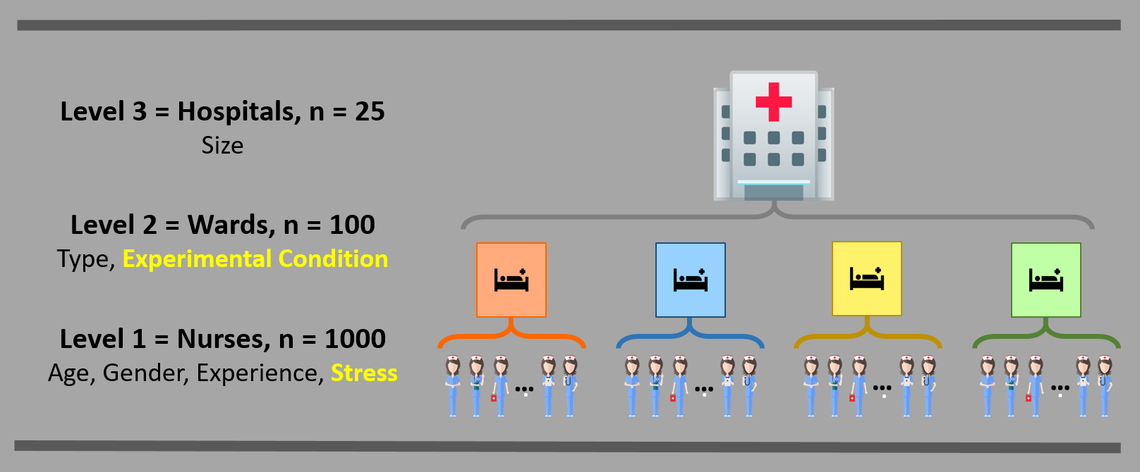
The nurses.sav file contains three-level simulated data from a hypothetical study on stress in hospitals. The data are from nurses working in wards nested within hospitals. It is a cluster-randomized experiment. In each of 25 hospitals, four wards are selected and randomly assigned to an experimental and a control condition. In the experimental condition, a training program is offered to all nurses to cope with job-related stress. After the program is completed, a sample of about 10 nurses from each ward is given a test that measures job-related stress. Additional variables (covariates) are: nurse age (years), nurse experience (years), nurse gender (0=male, 1 = female), type of ward (0=general care, 1=special care), and hospital size (0=small, 1 = medium, 2=large). The data have been generated to illustrate three-level analysis with a random slope for the effect of the intervention.
Here the data is read in and the SPSS variables with labels are converted to \(R\) factors.
df_raw <- haven::read_spss("data/Nurses.sav") %>%
  haven::as_factor() %>%             # retain the labels from SPSS --> factor
  haven::zap_label()
6.1.1 Unique Identifiers
All standardized (starts with “Z”) and mean centered (starts with “C”) variables will be remove so that their creation may be shown later. A new indicator varible for nurses with be created by combining the hospital, ward, and nurse indicators. Having a unique, distinct identifier variable for each of the units on lower (Level 1 and 2) levels is helpful for multilevel anlayses.
df_nurse <- df_raw %>%
  dplyr::mutate(genderF = factor(gender,
                                 labels = c("Male", "Female"))) %>% # apply factor labels
  dplyr::mutate(id = paste(hospital, ward, nurse,
                           sep = "_") %>%                                   # unique id for each nurse
                  factor()) %>%                                             # declare id is a factor
  dplyr::mutate_at(vars(hospital, ward,
                        wardid, nurse), factor) %>%                         # declare to be factors
  dplyr::mutate(age = age %>% as.character %>% as.numeric) %>%              # declare to be numeric
  dplyr::select(id, wardid, nurse, ward, hospital,
                age, gender, genderF, experien,
                wardtype, hospsize,
                expcon, stress)                                             # reduce variables included

tibble::glimpse(df_nurse)
Rows: 1,000
Columns: 13
$ id <fct> 1_1_1, 1_1_2, 1_1_3, 1_1_4, 1_1_5, 1_1_6, 1_1_7, 1_1_8, 1_1_9…
$ wardid <fct> 11, 11, 11, 11, 11, 11, 11, 11, 11, 12, 12, 12, 12, 12, 12, 1…
$ nurse <fct> 1, 2, 3, 4, 5, 6, 7, 8, 9, 10, 11, 12, 13, 14, 15, 16, 17, 18…
$ ward <fct> 1, 1, 1, 1, 1, 1, 1, 1, 1, 2, 2, 2, 2, 2, 2, 2, 2, 2, 3, 3, 3…
$ hospital <fct> 1, 1, 1, 1, 1, 1, 1, 1, 1, 1, 1, 1, 1, 1, 1, 1, 1, 1, 1, 1, 1…
$ age <dbl> 36, 45, 32, 57, 46, 60, 23, 32, 60, 45, 57, 47, 32, 42, 42, 5…
$ gender <dbl> 0, 0, 0, 1, 1, 1, 1, 1, 0, 0, 1, 0, 1, 1, 1, 1, 0, 1, 1, 0, 1…
$ genderF <fct> Male, Male, Male, Female, Female, Female, Female, Female, Mal…
$ experien <dbl> 11, 20, 7, 25, 22, 22, 13, 13, 17, 21, 24, 24, 14, 13, 17, 20…
$ wardtype <fct> general care, general care, general care, general care, gener…
$ hospsize <fct> large, large, large, large, large, large, large, large, large…
$ expcon <fct> experiment, experiment, experiment, experiment, experiment, e…
$ stress <dbl> 7, 7, 7, 6, 6, 6, 6, 7, 7, 6, 6, 6, 6, 6, 6, 5, 5, 6, 5, 5, 4…6.1.2 Centering Variables
When variables are involved in an interaction, it may be advantageous to center the variables. Hox, Moerbeek, and Van de Schoot (2017) covers this in chapter 4.
To center categorical variables:
1. Convert then to integers, starting with zero: \(0, 1, \dots\)
2. Subtract the mean
df_nurse %>%
  dplyr::mutate(expconN    = as.numeric(expcon)   - 1) %>%  # Numeric Version of experimental condition
  dplyr::mutate(hospsizeN  = as.numeric(hospsize) - 1) %>%  # Numeric Version of hospital size
  dplyr::select(expcon, expconN, hospsize, hospsizeN) %>%
  summary()
expcon expconN hospsize hospsizeN
control :496 Min. :0.000 small :374 Min. :0.000
experiment:504 1st Qu.:0.000 medium:476 1st Qu.:0.000
Median :1.000 large :150 Median :1.000
Mean :0.504 Mean :0.776
3rd Qu.:1.000 3rd Qu.:1.000
Max. :1.000 Max. :2.000 df_nurse <- df_nurse %>%
dplyr::mutate(expconN = as.numeric(expcon) - 1) %>% # Numeric Version of experimental condition
dplyr::mutate(hospsizeN = as.numeric(hospsize) - 1) %>% # Numeric Version of hospital size
dplyr::mutate(expconNG = expconN - 0.504) %>% # Grand-Mean Centered version of experimental condition
dplyr::mutate(hospsizeNG = hospsizeN - 0.776) # Grand-Mean Centered version of ehospital size expconNG
expcon -0.504 0.496
control 496 0
experiment 0 504 hospsizeNG
hospsize -0.776 0.224 1.224
small 374 0 0
medium 0 476 0
large 0 0 1506.2 Exploratory Data Analysis
6.2.1 Summarize Descriptive Statistics
Most posters, journal articles, and reports start with a table of descriptive statistics. Since it tends to come first, this type of table is often refereed to as Table 1.
df_nurse %>%
apaSupp::tab_desc(caption = "Descriptive statistics for continuous variables, aggregate over entire sample")NA | M | SD | min | Q1 | Mdn | Q3 | max | |
|---|---|---|---|---|---|---|---|---|
age | 0 | 43.01 | 12.04 | 23.00 | 33.00 | 43.00 | 53.00 | 64.00 |
gender | 0 | 0.73 | 0.44 | 0.00 | 0.00 | 1.00 | 1.00 | 1.00 |
experien | 0 | 17.06 | 6.04 | 1.00 | 13.00 | 17.00 | 21.00 | 38.00 |
stress | 0 | 4.98 | 0.98 | 1.00 | 4.00 | 5.00 | 6.00 | 7.00 |
expconN | 0 | 0.50 | 0.50 | 0.00 | 0.00 | 1.00 | 1.00 | 1.00 |
hospsizeN | 0 | 0.78 | 0.69 | 0.00 | 0.00 | 1.00 | 1.00 | 2.00 |
expconNG | 0 | -0.00 | 0.50 | -0.50 | -0.50 | 0.50 | 0.50 | 0.50 |
hospsizeNG | 0 | -0.00 | 0.69 | -0.78 | -0.78 | 0.22 | 0.22 | 1.22 |
Note. N = 1000. NA = not available or missing; Mdn = median; Q1 = 25th percentile; Q3 = 75th percentile. | ||||||||
df_nurse %>%
  dplyr::select(expcon,
                "Nurse: Age" = age,
                "Nurse: Gender" = genderF,
                "Nurse: Experience" = experien,
                "Ward: Type" = wardtype,
                "Hospital: Size" = hospsize) %>%
  apaSupp::tab1(split = "expcon",
                caption = "Compare Intervention groups on five main variables",
                p_note = NA)
| Total | control | experiment | p-value |
|---|---|---|---|---|
Nurse: Age | 43.01 (12.04) | 43.32 (11.59) | 42.69 (12.48) | .411 |
Nurse: Gender | .661 | |||
Male | 265 (26.5%) | 135 (27.2%) | 130 (25.8%) | |
Female | 735 (73.5%) | 361 (72.8%) | 374 (74.2%) | |
Nurse: Experience | 17.06 (6.04) | 17.19 (5.81) | 16.93 (6.27) | .491 |
Ward: Type | 1.000 | |||
general care | 499 (49.9%) | 247 (49.8%) | 252 (50.0%) | |
special care | 501 (50.1%) | 249 (50.2%) | 252 (50.0%) | |
Hospital: Size | .993 | |||
small | 374 (37.4%) | 185 (37.3%) | 189 (37.5%) | |
medium | 476 (47.6%) | 237 (47.8%) | 239 (47.4%) | |
large | 150 (15.0%) | 74 (14.9%) | 76 (15.1%) | |
Note. Continuous variables are summarized with means (SD) and significant group differences assessed via independent t-tests. Categorical variables are summarized with counts (%) and significant group differences assessed via Chi-squared tests for independence. | ||||
The t-test performed by the apaSupp::tab1() function
will always assume independent groups and that HOV is not violated. This
may or may not be appropriate.
6.3 MLM: Null Model
In a Null, intercept-only, or Empty model, no predictors are included.
6.3.0.1 Fit the Model
Fit the model to the data, with both ML and REML.
fit_lmer_0_re <-
  lmerTest::lmer(stress ~ 1 +              # Fixed Intercept for all nurses
                   (1|hospital/ward),      # Random Intercepts for wards within hospitals
                 data = df_nurse,
                 REML = TRUE)              # fit via REML (the default) for ICC calculations

fit_lmer_0_ml <-
  lmerTest::lmer(stress ~ 1 +              # Fixed Intercept for all nurses
                   (1|hospital/ward),      # Random Intercepts for wards within hospitals
                 data = df_nurse,
REML = FALSE) # fit via ML for comparing FIXED effects inclusionapaSupp::tab_lmers(list("M0: Null, ML" = fit_lmer_0_ml,
"M0: Null, REML" = fit_lmer_0_re),
var_labels = c("ward:hospital.var__(Intercept)" = "Var: Between Wards",
"hospital.var__(Intercept)" = "Var: Between Hospitals",
"Residual.var__Observation" = "Var: Between Nurses"),
caption = "NULL Model: different estimation methods",
p_note = "apa3",
general_note = "The estimates of fixed effects housl be near identical, but the estimates of random effects may differ slightly. The ICC should be calculated on the REML fit Null model.")
| M0: Null, ML | M0: Null, REML | ||||
|---|---|---|---|---|---|---|
Variable | b | (SE) | p | b | (SE) | p |
(Intercept) | 5.00 | (0.11) | < .001*** | 5.00 | (0.11) | < .001*** |
Var: Between Wards | 0.49 | 0.49 | ||||
Var: Between Hospitals | 0.16 | 0.17 | ||||
Var: Between Nurses | 0.30 | 0.30 | ||||
AIC | 1,950 | 1,953 | ||||
BIC | 1,970 | 1,973 | ||||
Log-likelihood | -971 | -972 | ||||
Note. The estimates of fixed effects housl be near identical, but the estimates of random effects may differ slightly. The ICC should be calculated on the REML fit Null model. | ||||||
*** p < .001. | ||||||
6.4 Estimate the ICC
The ICC is calculated by dividing the between-group-variance (random intercept variance) by the total variance (i.e. sum of between-group-variance and within-group (residual) variance).
 Groups        Name        Std.Dev.
 ward:hospital (Intercept) 0.69916
 hospital      (Intercept) 0.41749
Residual 0.54887 Groups Name Variance Std.Dev.
ward:hospital (Intercept) 0.489 0.699
hospital (Intercept) 0.174 0.417
Residual 0.301 0.549 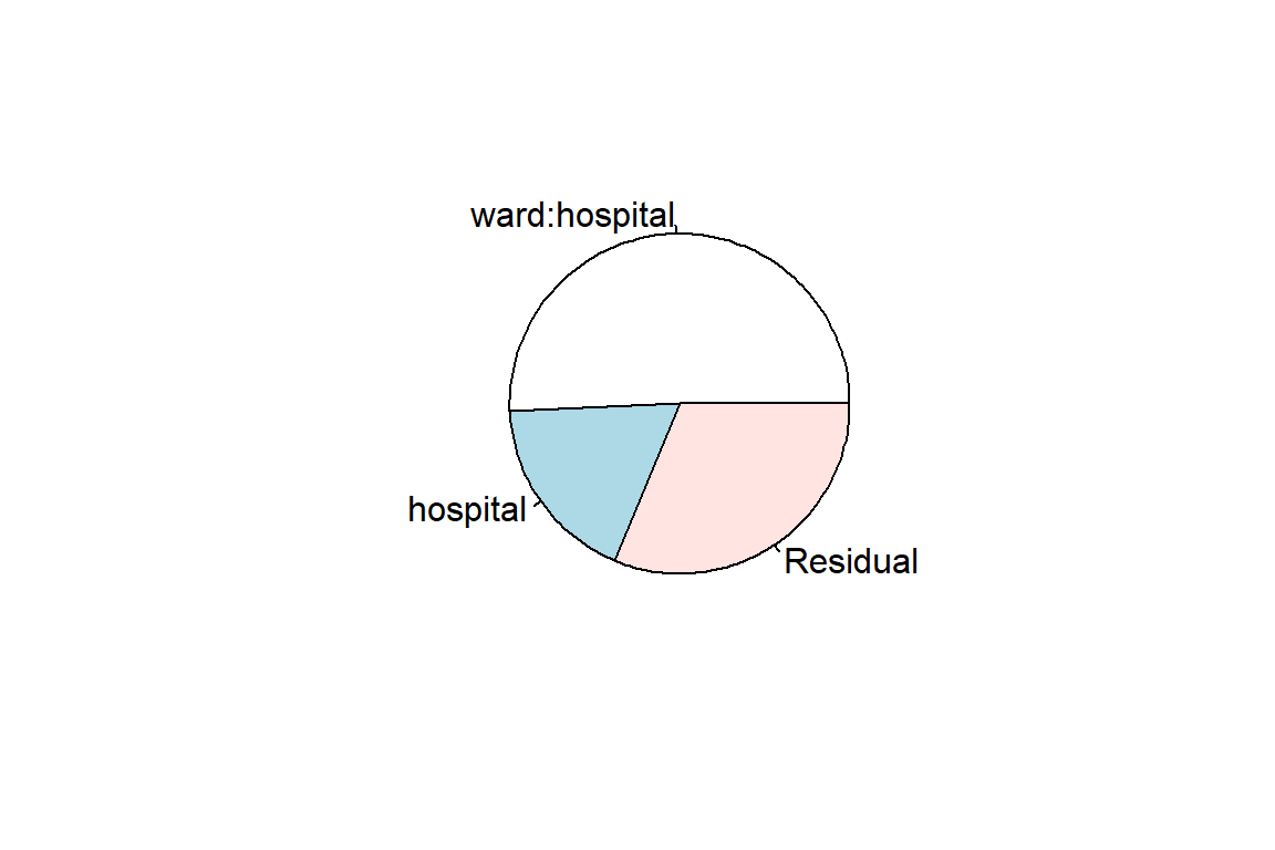
The performance package has a few really helpful funcitons:
 Groups        Name        Std.Dev.
 ward:hospital (Intercept) 0.69916
 hospital      (Intercept) 0.41749
Residual 0.54887 $var.fixed
[1] 0
$var.random
[1] 0.6631239
$var.residual
[1] 0.3012569
$var.distribution
[1] 0.3012569
$var.dispersion
[1] 0
$var.intercept
ward:hospital hospital
0.4888231 0.1743008 \[ \begin{align*} \text{hospitals} \rightarrow \; & \sigma^2_{v0} = 0.417^2 = 0.174\\ \text{wards within hospitals} \rightarrow \; & \sigma^2_{u0} = 0.699^2 = 0.489\\ \text{nurses within wards within hospitals} \rightarrow \; & \sigma^2_{e} = 0.549^2 = 0.301\\ \end{align*} \]
Intraclass Correlation (ICC) Formula, 3 level model - Davis and Scott Method \[ \overbrace{\rho_{mid}}^{\text{ICC}\atop\text{at level 2}} = \frac{\overbrace{\sigma^2_{u0}}^{\text{Random Intercept}\atop\text{Variance Level 2}}} {\underbrace{\sigma^2_{v0}+\sigma^2_{u0}+\sigma^2_{e}}_{\text{Total}\atop\text{Variance}}} \tag{Hox 2.16} \] \[ \overbrace{\rho_{top}}^{\text{ICC}\atop\text{ at level 3}} = \frac{\overbrace{\sigma^2_{v0}}^{\text{Random Intercept}\atop\text{Variance Level 3}}} {\underbrace{\sigma^2_{v0}+\sigma^2_{u0}+\sigma^2_{e}}_{\text{Total}\atop\text{Variance}}} \tag{Hox 2.17} \]
[1] 0.5072614[1] 0.1804979For more than two levels, the ‘performance::icc()’ function computes ICC’s by the Davis and Scott method.
# Intraclass Correlation Coefficient

    Adjusted ICC: 0.688
Unadjusted ICC: 0.688# ICC by Group
Group | ICC
---------------------
ward:hospital | 0.507
hospital | 0.181The proportion of variance in nurse stress level is 0.51 at the ward level and 0.18 at the hospital level, for a total of 0.69.
To test if the three level model is justified statistically, compare the null models with and without the nesting of wards in hospitals.
fit_lmer_0_re_2level <-
  lmerTest::lmer(stress ~ 1 + (1|wardid),  # each hospital contains several wards
                 data = df_nurse,
REML = TRUE) # fit via REML (the default) for ICC calculationsEst | (SE) | p | |
|---|---|---|---|
(Intercept) | 5.00 | (0.08) | < .001*** |
wardid.var__(Intercept) | 0.66 | ||
Residual.var__Observation | 0.30 | ||
Note. Est = estimated regresssion coefficient for fixed effects and varaince/covariance estimates for random effects. p = significance from Wald t-test for parameter estimate using Satterthwaite's method for degrees of freedom. | |||
* p < .05. ** p < .01. *** p < .001. | |||
6.5 xxx - Sarah needs to fix this table! - xxx
apaSupp::tab_lmers(list("2 levels" = fit_lmer_0_re_2level,
                        "3 levels" = fit_lmer_0_re),
                   caption = "MLM: Two or Three Levels?")
| 2 levels | 3 levels | ||||
|---|---|---|---|---|---|---|
Variable | b | (SE) | p | b | (SE) | p |
(Intercept) | 5.00 | (0.08) | < .001*** | 5.00 | (0.11) | < .001*** |
wardid.var__(Intercept) | 0.66 | |||||
Residual.var__Observation | 0.30 | 0.30 | ||||
ward:hospital.var__(Intercept) | 0.49 | |||||
hospital.var__(Intercept) | 0.17 | |||||
AIC | 1,958 | 1,953 | ||||
BIC | 1,973 | 1,973 | ||||
Log-likelihood | -976 | -972 | ||||
Note. | ||||||
* p < .05. ** p < .01. *** p < .001. | ||||||
Model | AIC | BIC | RMSE |
| |
|---|---|---|---|---|---|
Conditional | Marginal | ||||
2 levels | 1955.29 | 1970.01 | 0.52 | .686 | < .001 |
3 levels | 1950.38 | 1970.01 | 0.52 | .688 | < .001 |
Note. Larger values indicated better performance. Smaller values indicated better performance for Akaike's Information Criteria (AIC), Bayesian information criteria (BIC), and Root Mean Squared Error (RMSE). | |||||
The deviance test or likelihood-ratio test shows that the inclusion of the nesting of wards within hospitals better explains the variance in nurse stress levels.
Data: df_nurse
Models:
fit_lmer_0_re_2level: stress ~ 1 + (1 | wardid)
fit_lmer_0_re: stress ~ 1 + (1 | hospital/ward)
                     npar    AIC    BIC  logLik -2*log(L)  Chisq Df Pr(>Chisq)
fit_lmer_0_re_2level    3 1958.4 1973.2 -976.21    1952.4
fit_lmer_0_re           4 1953.0 1972.6 -972.48    1945.0 7.4738  1    0.00626

fit_lmer_0_re_2level
fit_lmer_0_re        **
---
Signif. codes:  0 '***' 0.001 '**' 0.01 '*' 0.05 '.' 0.1 ' ' 1
Single-term deletion is alonther way to determine significance of random effects.
ANOVA-like table for random-effects: Single term deletions

Model:
stress ~ (1 | ward:hospital) + (1 | hospital)
                    npar   logLik    AIC    LRT Df Pr(>Chisq)
<none>                 4  -972.48 1953.0
(1 | ward:hospital)    3 -1267.32 2540.6 589.69  1    < 2e-16 ***
(1 | hospital)         3  -976.21 1958.4   7.47  1    0.00626 **
---
Signif. codes:  0 '***' 0.001 '**' 0.01 '*' 0.05 '.' 0.1 ' ' 1
6.6 MLM: Add Fixed Effects
6.6.1 Fit the Model
Hox, Moerbeek, and Van de Schoot (2017), page 22:
“In this example, the variable
expconis of main interest, and the other variables are covariates. Their funciton is to control for differences between the groups, which can occur even if randomization is used, especially with small samples, and to explain variance in the outcome variable stress. To the extent that these variables successfully explain the variance, the power of the test for the effect ofexpconwill be increased.”
fit_lmer_1_ml <-
  lmerTest::lmer(stress ~ expcon +             # experimental condition = CATEGORICAL FACTOR
                   age + gender + experien +   # level 1 covariates
                   wardtype +                  # level 2 covariates
                   hospsize +                  # level 3 covariates, hospital size = CATEGORICAL FACTOR
                   (1|hospital/ward),          # Random Intercepts for wards within hospitals
                 data = df_nurse,
REML = FALSE) # fit via ML for nested FIXED effectsapaSupp::tab_lmers(list("M0: null" = fit_lmer_0_ml,
"M1: fixed pred" = fit_lmer_1_ml),
caption = "Nested Models: Fixed effects via ML")
| M0: null | M1: fixed pred | ||||
|---|---|---|---|---|---|---|
Variable | b | (SE) | p | b | (SE) | p |
(Intercept) | 5.00 | (0.11) | < .001*** | 5.38 | (0.18) | < .001*** |
expcon | ||||||
control | — | — | ||||
experiment | -0.70 | (0.12) | < .001*** | |||
age | 0.02 | (0.00) | < .001*** | |||
gender | -0.45 | (0.03) | < .001*** | |||
experien | -0.06 | (0.00) | < .001*** | |||
wardtype | ||||||
general care | — | — | ||||
special care | 0.05 | (0.12) | .668 | |||
hospsize | ||||||
small | — | — | ||||
medium | 0.49 | (0.19) | .016* | |||
large | 0.90 | (0.26) | .002** | |||
ward:hospital.var__(Intercept) | 0.49 | 0.33 | ||||
hospital.var__(Intercept) | 0.16 | 0.10 | ||||
Residual.var__Observation | 0.30 | 0.22 | ||||
AIC | 1,950 | 1,626 | ||||
BIC | 1,970 | 1,680 | ||||
Log-likelihood | -971 | -802 | ||||
Note. | ||||||
* p < .05. ** p < .01. *** p < .001. | ||||||
6.6.2 Assess Significance
Data: df_nurse
Models:
fit_lmer_0_ml: stress ~ 1 + (1 | hospital/ward)
fit_lmer_1_ml: stress ~ expcon + age + gender + experien + wardtype + hospsize + (1 | hospital/ward)
              npar    AIC    BIC  logLik -2*log(L)  Chisq Df Pr(>Chisq)
fit_lmer_0_ml    4 1950.4 1970.0 -971.18    1942.4
fit_lmer_1_ml   11 1626.3 1680.3 -802.16    1604.3 338.04  7  < 2.2e-16 ***
---
Signif. codes:  0 '***' 0.001 '**' 0.01 '*' 0.05 '.' 0.1 ' ' 1
It is clear that inclusion of these fixed, main effects improves the model’s fit, but it is questionable that the type of ward is significant (Wald test is non-significant). Rather than test it directly, we will leave it in the model. This is common practice to show that an expected variable is not significant.
6.6.3 Centering Variables
Because we will will find that the experimental condition is moderated by hospital size (in other words there is a significant interaction between expcon and hospsize), Hox, Moerbeek, and Van de Schoot (2017) presents the models fit with centered values for these two variables. Let us see how this changes the model.
(1) Experimental Condition
Experimental conditon is a BINARY or two-level factor.
When it is alternatively coded as a numeric, continuous variable taking the values of zero (\(0\)) for the reference category and one (\(1\)) for the other category, the model estimates are exactly the same, including the paramters for the variables and the intercept, AND the model fit statistics.
When the numeric, continuous variable is further grand-mean centered by additionally subtraction the MEAN of the numberic version, the value of the intercept is the only estimate that changes.
fit_lmer_1a_ml <-
  lmerTest::lmer(stress ~ expconN +            # experimental condition = CONTINUOUS CODED 0/1
                   age + gender + experien +
                   wardtype +
                   hospsize +                 # hospital size = CATEGORICAL FACTOR
                   (1|hospital/ward),
                 data = df_nurse,
                 REML = FALSE)

fit_lmer_1b_ml <-
  lmerTest::lmer(stress ~ expconNG +           # experimental condition = CONTINUOUS GRAND-MEAN CENTERED
                   age + gender + experien +
                   wardtype +
                   hospsize +                  # hospital size = CATEGORICAL FACTOR
                   (1|hospital/ward),
                 data = df_nurse,
REML = FALSE) apaSupp::tab_lmers(list("Factor" = fit_lmer_1_ml,
"0 vs 1" = fit_lmer_1a_ml,
"Centered" = fit_lmer_1b_ml),
narrow = TRUE,
caption = "MLM: Model 1 - Expereimental Condiditon Coding (2-levels)",
general_note = "These models only differ in how the experimental condition variable is coded.")
| Factor | 0 vs 1 | Centered | |||
|---|---|---|---|---|---|---|
Variable | b | (SE) | b | (SE) | b | (SE) |
(Intercept) | 5.38 | (0.18) *** | 5.38 | (0.18) *** | 5.03 | (0.17) *** |
expcon | ||||||
control | — | — | ||||
experiment | -0.70 | (0.12) *** | ||||
age | 0.02 | (0.00) *** | 0.02 | (0.00) *** | 0.02 | (0.00) *** |
gender | -0.45 | (0.03) *** | -0.45 | (0.03) *** | -0.45 | (0.03) *** |
experien | -0.06 | (0.00) *** | -0.06 | (0.00) *** | -0.06 | (0.00) *** |
wardtype | ||||||
general care | — | — | — | — | — | — |
special care | 0.05 | (0.12) | 0.05 | (0.12) | 0.05 | (0.12) |
hospsize | ||||||
small | — | — | — | — | — | — |
medium | 0.49 | (0.19) * | 0.49 | (0.19) * | 0.49 | (0.19) * |
large | 0.90 | (0.26) ** | 0.90 | (0.26) ** | 0.90 | (0.26) ** |
expconN | -0.70 | (0.12) *** | ||||
expconNG | -0.70 | (0.12) *** | ||||
ward:hospital.var__(Intercept) | 0.33 | 0.33 | 0.33 | |||
hospital.var__(Intercept) | 0.10 | 0.10 | 0.10 | |||
Residual.var__Observation | 0.22 | 0.22 | 0.22 | |||
AIC | 1,626 | 1,626 | 1,626 | |||
BIC | 1,680 | 1,680 | 1,680 | |||
Log-likelihood | -802 | -802 | -802 | |||
Note. These models only differ in how the experimental condition variable is coded. | ||||||
* p < .05. ** p < .01. *** p < .001. | ||||||
(2) Hospital Size
Experimental conditon is a three-level factor.
When it is alternatively coded as a numeric, continuous variables taking the values of whole numbers, starting with zero (\(0, 1, 2, \dots\)), the model there will only be ONE parameter estimated instead of several (one less than the number of categories). This is becuase the levels are treated as being equally different from each other in terms of the outcome. This treats the effect of the categorical variable as if it is linear, which may or may not be appropriate. User beware!
When the numeric, continuous variable is further grand-mean centered by additionally subtraction the MEAN of the numberic version, the value of the intercept is the only estimate that changes.
fit_lmer_1c_ml <-
  lmerTest::lmer(stress ~ expconNG +           # experimental condition = CONTINUOUS GRAND-MEAN CENTERED
                   age + gender + experien +
                   wardtype +
                   hospsizeN +                 # hospital size = CONTINUOUS CODED 0/1
                   (1|hospital/ward),
                 data = df_nurse,
                 REML = FALSE)

fit_lmer_1d_ml <-
  lmerTest::lmer(stress ~ expconNG +           # experimental condition = CONTINUOUS GRAND-MEAN CENTERED
                   age + gender + experien +
                   wardtype +
                   hospsizeNG +                # hospital size = CONTINUOUS GRAND-MEAN CENTERED
                   (1|hospital/ward),
                 data = df_nurse,
REML = FALSE)apaSupp::tab_lmers(list("Factor" = fit_lmer_1b_ml,
"0 vs 1" = fit_lmer_1c_ml,
"Centered" = fit_lmer_1d_ml),
narrow = TRUE,
caption = "MLM: Model 1 - Hospital Coding (3-levels)",
general_note = "These models only differ in how the hospital size variable is coded.")
| Factor | 0 vs 1 | Centered | |||
|---|---|---|---|---|---|---|
Variable | b | (SE) | b | (SE) | b | (SE) |
(Intercept) | 5.03 | (0.17) *** | 5.04 | (0.16) *** | 5.40 | (0.12) *** |
expconNG | -0.70 | (0.12) *** | -0.70 | (0.12) *** | -0.70 | (0.12) *** |
age | 0.02 | (0.00) *** | 0.02 | (0.00) *** | 0.02 | (0.00) *** |
gender | -0.45 | (0.03) *** | -0.45 | (0.03) *** | -0.45 | (0.03) *** |
experien | -0.06 | (0.00) *** | -0.06 | (0.00) *** | -0.06 | (0.00) *** |
wardtype | ||||||
general care | — | — | — | — | — | — |
special care | 0.05 | (0.12) | 0.05 | (0.12) | 0.05 | (0.12) |
hospsize | ||||||
small | — | — | ||||
medium | 0.49 | (0.19) * | ||||
large | 0.90 | (0.26) ** | ||||
hospsizeN | 0.46 | (0.12) ** | ||||
hospsizeNG | 0.46 | (0.12) ** | ||||
ward:hospital.var__(Intercept) | 0.33 | 0.33 | 0.33 | |||
hospital.var__(Intercept) | 0.10 | 0.10 | 0.10 | |||
Residual.var__Observation | 0.22 | 0.22 | 0.22 | |||
AIC | 1,626 | 1,624 | 1,624 | |||
BIC | 1,680 | 1,673 | 1,673 | |||
Log-likelihood | -802 | -802 | -802 | |||
Note. These models only differ in how the hospital size variable is coded. | ||||||
* p < .05. ** p < .01. *** p < .001. | ||||||
6.7 MLM: Add Random Slope
Hox, Moerbeek, and Van de Schoot (2017), page 22:
“Although logically we can test if explanatory variables at the first level have random coefficients (slopes) at the second or third level, and if explanatory variables at teh second level have random coefficients (slopes) at the third level, these possibilities are not pursued. We DO test a model with a random coefficient (slope) for
expconat the third level, where there turns out to be significant slope variation.”
6.7.1 Fit the Model
fit_lmer_1d_re <-
  lmerTest::lmer(stress ~ expconNG +            # experimental condition = CONTINUOUS GRAND-MEAN CENTERED
                   age + gender + experien +    # level 1 covariates
                   wardtype +                   # level 2 covariate
                   hospsizeNG +                 # level 3 covariate, hospital size = CONTINUOUS GRAND-MEAN CENTERED
                   (1|hospital/ward),           # Random Intercepts for wards within hospitals
                 data = df_nurse,
                 REML = TRUE)                   # fit via REML for nested Random Effects

fit_lmer_2_re <-
  lmerTest::lmer(stress ~ expconNG +             # experimental condition = CONTINUOUS GRAND-MEAN CENTERED
                   age + gender + experien +     # level 1 covariates
                   wardtype +                    # level 2 covariate
                   hospsizeNG +                  # level 3 covariate, hospital size = CONTINUOUS GRAND-MEAN CENTERED
                   (1|hospital/ward) +           # Random Intercepts for wards within hospitals
                   (0 + expconNG|hospital),      # RANDOM SLOPES for exp cond within hospital (does not vary witin a ward!)
                 data = df_nurse,
                 REML = TRUE)                    # fit via REML for nested Random Effects
6.8 xxx – Sarah needs to fix this table – XXX
| M1: RI | M2: RIAS | ||||
|---|---|---|---|---|---|---|
Variable | b | (SE) | p | b | (SE) | p |
(Intercept) | 5.40 | (0.12) | < .001*** | 5.39 | (0.11) | < .001*** |
expconNG | -0.70 | (0.12) | < .001*** | -0.70 | (0.18) | < .001*** |
age | 0.02 | (0.00) | < .001*** | 0.02 | (0.00) | < .001*** |
gender | -0.45 | (0.03) | < .001*** | -0.45 | (0.03) | < .001*** |
experien | -0.06 | (0.00) | < .001*** | -0.06 | (0.00) | < .001*** |
wardtype | ||||||
general care | — | — | — | — | ||
special care | 0.05 | (0.12) | .673 | 0.05 | (0.07) | .471 |
hospsizeNG | 0.46 | (0.13) | .002** | 0.46 | (0.13) | .002** |
ward:hospital.var__(Intercept) | 0.34 | |||||
hospital.var__(Intercept) | 0.11 | 0.17 | ||||
Residual.var__Observation | 0.22 | 0.22 | ||||
ward.hospital.var__(Intercept) | 0.11 | |||||
hospital.1.var__expconNG | 0.69 | |||||
AIC | 1,660 | 1,633 | ||||
BIC | 1,709 | 1,687 | ||||
Log-likelihood | -820 | -806 | ||||
Note. | ||||||
* p < .05. ** p < .01. *** p < .001. | ||||||
6.8.1 Assess Significance
Data: df_nurse
Models:
fit_lmer_1d_re: stress ~ expconNG + age + gender + experien + wardtype + hospsizeNG + (1 | hospital/ward)
fit_lmer_2_re: stress ~ expconNG + age + gender + experien + wardtype + hospsizeNG + (1 | hospital/ward) + (0 + expconNG | hospital)
               npar    AIC    BIC  logLik -2*log(L)  Chisq Df Pr(>Chisq)
fit_lmer_1d_re   10 1659.9 1709.0 -819.94    1639.9
fit_lmer_2_re    11 1633.2 1687.2 -805.59    1611.2 28.708  1  8.417e-08 ***
---
Signif. codes:  0 '***' 0.001 '**' 0.01 '*' 0.05 '.' 0.1 ' ' 1
The inclusion of a random slope effect for the experimental condition expcon significantly improves the models’s fit, thus is should be retained.
6.9 MLM: Add Cross-Level Interaction
Hox, Moerbeek, and Van de Schoot (2017), page 22:
“The varying slope can be predicted by adding a cross-level interaction between the variables
expconandhospsize. In view of this interaction, the variablesexpconandhospsizehave been centered on tehir overal means.”
6.9.1 Fit the Model
fit_lmer_2_ml <-
  lmerTest::lmer(stress ~ expconNG +           # experimental condition = CONTINUOUS GRAND-MEAN CENTERED
                   age + gender + experien +   # level 1 covariates
                   wardtype +                  # level 2 covariate
                   hospsizeNG +                # level 3 covariate, hospital size = CONTINUOUS GRAND-MEAN CENTERED
                   (1|hospital/ward) +         # Random Intercepts for wards within hospitals
                   (0 + expconNG|hospital),    # RANDOM SLOPES for exp cond within hospital (does not vary witin a ward!)
                 data = df_nurse,
                 REML = FALSE)                 # fit via ML for nested FIXED Effects

fit_lmer_3_ml <-
  lmerTest::lmer(stress ~ expconNG +           # experimental condition = CONTINUOUS GRAND-MEAN CENTERED
                   age + gender + experien +   # level 1 covariates
                   wardtype +                  # level 2 covariate
                   hospsizeNG +                # level 3 covariate, hospital size = CONTINUOUS GRAND-MEAN CENTERED
                   expconNG*hospsizeNG +       # CROSS-LEVEL interaction
                   (1|hospital/ward) +         # Random Intercepts for wards within hospitals
                   (0 + expconNG|hospital),    # RANDOM SLOPES for exp cond within hospital (does not vary within a ward!)
                 data = df_nurse,
REML = FALSE) # fit via ML for nested FIXED EffectsapaSupp::tab_lmers(list("M2: RAIS" = fit_lmer_2_ml,
"M3: Xlevel Int" = fit_lmer_3_ml),
caption = "Nested Models: Fixed Cross-Level Interaction via ML")
| M2: RAIS | M3: Xlevel Int | ||||
|---|---|---|---|---|---|---|
Variable | b | (SE) | p | b | (SE) | p |
(Intercept) | 5.39 | (0.11) | < .001*** | 5.39 | (0.11) | < .001*** |
expconNG | -0.70 | (0.18) | < .001*** | -0.72 | (0.11) | < .001*** |
age | 0.02 | (0.00) | < .001*** | 0.02 | (0.00) | < .001*** |
gender | -0.46 | (0.03) | < .001*** | -0.46 | (0.03) | < .001*** |
experien | -0.06 | (0.00) | < .001*** | -0.06 | (0.00) | < .001*** |
wardtype | ||||||
general care | — | — | — | — | ||
special care | 0.05 | (0.07) | .466 | 0.05 | (0.07) | .466 |
hospsizeNG | 0.46 | (0.12) | .001** | 0.46 | (0.12) | .001** |
expconNG * hospsizeNG | 1.00 | (0.16) | < .001*** | |||
ward.hospital.var__(Intercept) | 0.11 | 0.11 | ||||
hospital.var__(Intercept) | 0.15 | 0.15 | ||||
hospital.1.var__expconNG | 0.66 | 0.18 | ||||
Residual.var__Observation | 0.22 | 0.22 | ||||
AIC | 1,597 | 1,576 | ||||
BIC | 1,651 | 1,635 | ||||
Log-likelihood | -788 | -776 | ||||
Note. | ||||||
* p < .05. ** p < .01. *** p < .001. | ||||||
6.9.2 Assess Significance
Data: df_nurse
Models:
fit_lmer_2_ml: stress ~ expconNG + age + gender + experien + wardtype + hospsizeNG + (1 | hospital/ward) + (0 + expconNG | hospital)
fit_lmer_3_ml: stress ~ expconNG + age + gender + experien + wardtype + hospsizeNG + expconNG * hospsizeNG + (1 | hospital/ward) + (0 + expconNG | hospital)
              npar    AIC    BIC  logLik -2*log(L)  Chisq Df Pr(>Chisq)
fit_lmer_2_ml   11 1597.5 1651.5 -787.74    1575.5
fit_lmer_3_ml   12 1576.1 1635.0 -776.03    1552.1 23.413  1  1.307e-06 ***
---
Signif. codes:  0 '***' 0.001 '**' 0.01 '*' 0.05 '.' 0.1 ' ' 1
There is evidence that hospital size moderated the effect of the intervention. We will want to plot the estimated marginal means to interpret the meaning of this interaction.
6.10 Final Model
6.10.1 Fit the model
The final model should be fit via REML.
I’m going to revert back to the factor versions of hospital size and experimental condition, but grand-mean center age and experience
# A tibble: 1 × 2
    age experien
  <dbl>    <dbl>
1  43.0     17.1
fit_lmer_final <-
lmerTest::lmer(stress ~ expcon + # experimental condition = CONTINUOUS GRAND-MEAN CENTERED
I(age - 43.01) + gender + I(experien - 17.06) + # level 1 covariates
wardtype + # level 2 covariate
hospsize + # level 3 covariate, hospital size = CONTINUOUS GRAND-MEAN CENTERED
expcon*hospsize + # CROSS-LEVEL interaction
(1|hospital/ward) + # Random Intercepts for wards within hospitals
(0 + expconNG|hospital), # RANDOM SLOPES for exp condition within hospital (does not vary within a ward!)
data = df_nurse,
REML = TRUE) # fit via REML for final model 6.10.2 Table of Estimated Parameters
Type III Analysis of Variance Table with Satterthwaite's method
                    Sum Sq Mean Sq NumDF  DenDF  F value    Pr(>F)
expcon               3.532   3.532     1  22.04  16.2512 0.0005573 ***
I(age - 43.01)      22.400  22.400     1 909.68 103.0680 < 2.2e-16 ***
gender              36.949  36.949     1 914.46 170.0117 < 2.2e-16 ***
I(experien - 17.06) 41.656  41.656     1 918.66 191.6692 < 2.2e-16 ***
wardtype             0.115   0.115     1  49.10   0.5278 0.4709777
hospsize             2.622   1.311     2  22.00   6.0321 0.0081539 **
expcon:hospsize      7.608   3.804     2  22.01  17.5040 2.822e-05 ***
---
Signif. codes: 0 '***' 0.001 '**' 0.01 '*' 0.05 '.' 0.1 ' ' 1Est | (SE) | p | |
|---|---|---|---|
(Intercept) | 5.70 | (0.19) | < .001*** |
expcon | |||
control | — | — | |
experiment | -1.55 | (0.20) | < .001*** |
I(age - 43.01) | 0.02 | (0.00) | < .001*** |
gender | -0.46 | (0.03) | < .001*** |
I(experien - 17.06) | -0.06 | (0.00) | < .001*** |
wardtype | |||
general care | — | — | |
special care | 0.05 | (0.07) | .471 |
hospsize | |||
small | — | — | |
medium | -0.07 | (0.24) | .772 |
large | -0.07 | (0.33) | .836 |
expcon * hospsize | |||
experiment * medium | 1.12 | (0.26) | < .001*** |
experiment * large | 1.94 | (0.35) | < .001*** |
ward.hospital.var__(Intercept) | 0.11 | ||
hospital.var__(Intercept) | 0.18 | ||
hospital.1.var__expconNG | 0.21 | ||
Residual.var__Observation | 0.22 | ||
Note. Est = estimated regresssion coefficient for fixed effects and varaince/covariance estimates for random effects. p = significance from Wald t-test for parameter estimate using Satterthwaite's method for degrees of freedom. | |||
* p < .05. ** p < .01. *** p < .001. | |||
Interpretation: After accounting for the a nurses’ age, gender, and experience, as well as the ward type, the effect of the intervention is moderated by hospital size, X2(1) = 23.41, p < .001,
6.10.3 Visualization: Estimated Marginal Means Plot
Although there are many variables in this model, only two are involved in any interaction(s). For this reason, we will choose to display the estimated marginal means across only experimental condition and hospital size. For this illustration, all other continuous predictors are taken to be at their mean and categorical predictors at their reference category.
6.10.3.1 Using interactions::interact_plot()
All Defaults:
interactions::cat_plot(model = fit_lmer_final,
                       pred = hospsize,          # main predictor/independent variable, for x-axis
                       modx = expcon,            # moderating independent variable, for different lines
                       interval = TRUE)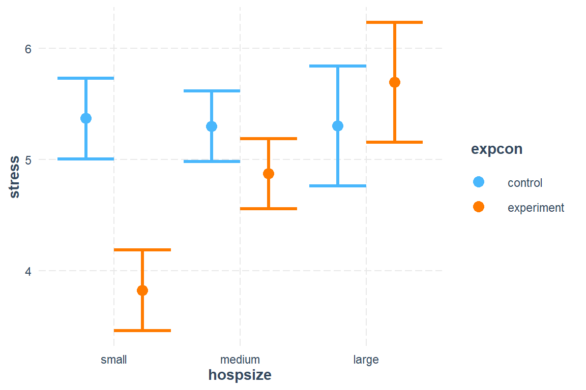
Look: We can make NASTY dynamite plots! DO NOT EVER USE THESE!
From the help menu: “Many applied researchers advise against this type of plot because it does not represent the distribution of the observed data or the uncertainty of the predictions very well.”
interactions::cat_plot(model = fit_lmer_final,
                       pred = hospsize,          # main predictor/independent variable, for x-axis
                       modx = expcon,            # moderating independent variable, for different lines
                       interval = TRUE,
                       geom = "bar")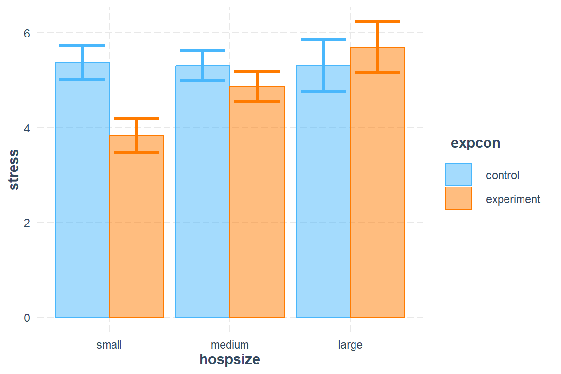
6.10.4 Post Hoc Pairwise Tests
When an interactions is between two categorical predictors, compare pairs of mean predictions.
hospsize = small:
contrast estimate SE df t.ratio p.value
control - experiment 1.545 0.196 21.9 7.898 <.0001
hospsize = medium:
contrast estimate SE df t.ratio p.value
control - experiment 0.427 0.170 22.0 2.518 0.0196
hospsize = large:
contrast estimate SE df t.ratio p.value
control - experiment -0.392 0.294 22.2 -1.332 0.1964
Results are averaged over the levels of: gender, wardtype
Degrees-of-freedom method: kenward-roger Interpretation: For hospitals that are small in size, the intervention does substantially decrease stress levels by 1.55 points, SE = 0.20, p <.001. For hospitals that are medium sizes, the intervention does decrease stress, but by a modest 0.43 points, SD = 0.17, p = .020. For large hospitals the intervention was not effective at reducing stress, p = .200.
6.10.5 Effect Sizes
From the help page for emmeans::eff_size:
For models having a single random effect, such as those fitted using lm; in that case, the stats::sigma() and stats::df.residual() functions may be useful for specifying sigma and edf.For models with **more than one random effect**,sigma` may be based on some combination of the random-effect variances.
Specifying edf can be rather un-intuitive but is also relatively un-critical; but the smaller the value, the wider the confidence intervals for effect size. The value of sqrt(2/edf) can be interpreted as the relative accuracy of sigma; for example, with edf = 50, \(\sqrt{\frac{2}{50}}\) = 0.2, meaning that sigma is accurate to plus or minus 20 percent. Note in an example below, we tried two different edf values as kind of a bracketing/sensitivity-analysis strategy. A value of Inf is allowable, in which case you are assuming that sigma is known exactly. Obviously, this narrows the confidence intervals for the effect sizes – unrealistically if in fact sigma is unknown.
6.10.5.1 Compute Standardized Mean Differences
FIRST: We need to compute the values to standardize by…“Sigma”.
Option 1) Pooled SD <– My favorite
- added all the model’s variance components
- took the standard deviation
[1] 0.8465793Option 2) SD of all stress levels for all participants
# A tibble: 1 × 1
`sd(stress)`
<dbl>
1 0.980Option 3) SD of stress levels for participants in the control group
# A tibble: 1 × 1
`sd(stress)`
<dbl>
1 0.724SECOND: We need to compute the numeric scalar that specifies the equivalent degrees of freedom for the sigma.
This is a way of specifying the uncertainty in sigma, in that we regard our estimate of sigma^2 as being proportional to a chi-square random variable with edf degrees of freedom. (edf should not be confused with the df argument that may be passed via … to specify the degrees of freedom to use in t statistics and confidence intervals.)
This value has an effect the SE and confidence intervals, which I suggest you do not report, so just throw any old number in there ;)
fit_lmer_final %>%
  emmeans::emmeans(~ expcon | hospsize) %>%
pairs() %>%
data.frame() %>%
dplyr::mutate(smd = estimate/totalSD) %>%
dplyr::select(contrast, hospsize, estimate, SE, p.value, smd) %>%
flextable::flextable() %>%
apaSupp::theme_apa(caption = "Follow-up Compairsons Between Intervention Groups by Hospital Size")contrast | hospsize | estimate | SE | p.value | smd |
|---|---|---|---|---|---|
control - experiment | small | 1.55 | 0.20 | 0.00 | 1.83 |
control - experiment | medium | 0.43 | 0.17 | 0.02 | 0.50 |
control - experiment | large | -0.39 | 0.29 | 0.20 | -0.46 |
FULL INTERPRETATION: After accounting for the a nurses’ age, gender, and experience, as well as the ward type, the effect of the intervention is moderated by hospital size, F(2, 22) = 17.50, p < .001. For hospitals that are small in size, the intervention does substantially decrease stress levels by 1.55 points, SE = 0.20, p <.001, Cohen’s d = 1.83. For hospitals that are medium sizes, the intervention does decrease stress, but by a modest 0.43 points, SD = 0.17, p = .020, Cohen’s d = 0.51. For large hospitals the intervention was not effective at reducing stress, p = .200.
Adding more options:
interactions::cat_plot(fit_lmer_final,
                       pred = "hospsize",
                       modx = "expcon",
                       interval = TRUE,
                       y.label = "Estimated Marginal Mean Norse's Stress Score",
                       x.label = "Hospital Size",
                       legend.main = "Condition:",
                       modx.labels = c("Control", "Intervention"),
                       colors = c("gray40", "black"),
                       point.shape = TRUE,
                       pred.point.size = 5,
                       dodge.width = .3,
                       errorbar.width = .25,
                       geom = "line") +
  theme_bw() +
  theme(legend.key.width = unit(2, "cm"),
        legend.background = element_rect(color = "Black"),
        legend.position = c(1, 0),
        legend.justification = c(1.1, -0.1)) +
scale_y_continuous(breaks = seq(from = 0, to = 10, by = 1)) 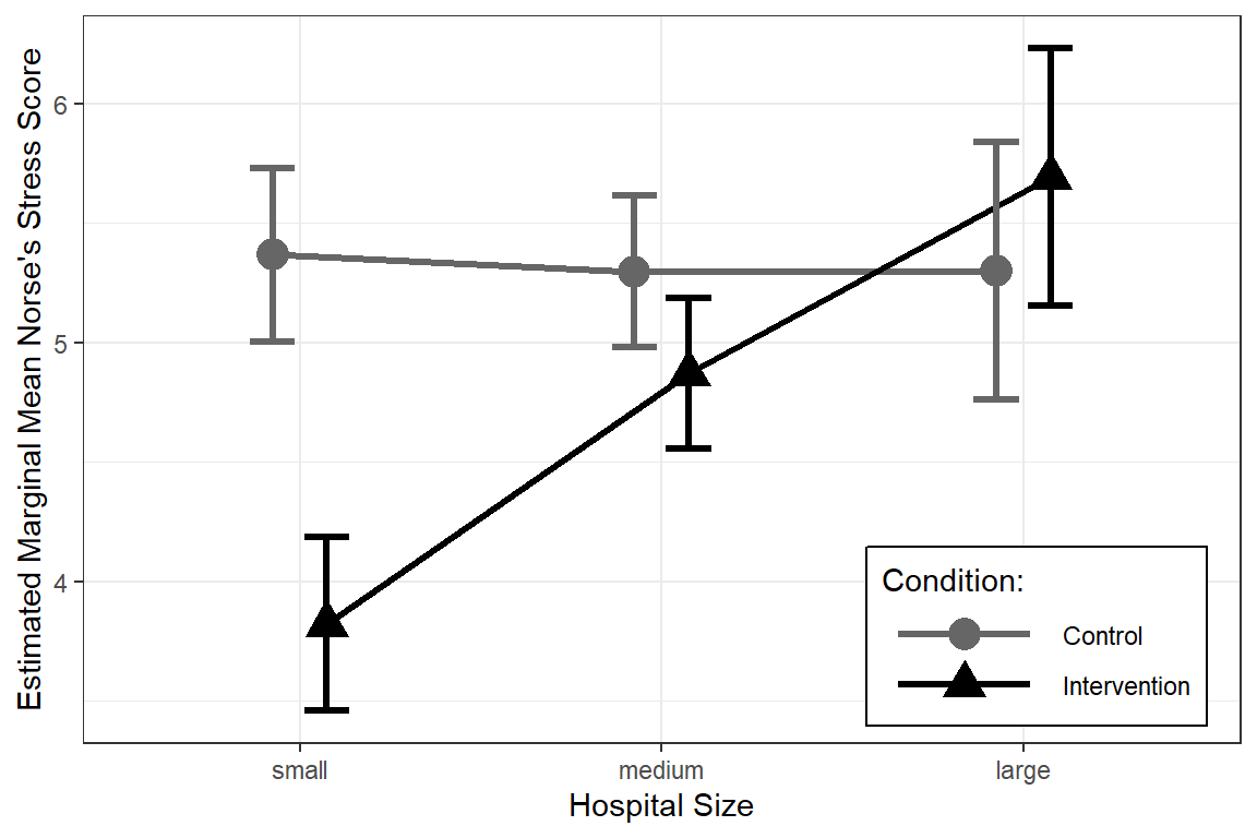
6.10.5.2 Using sjPlot::plot_model()
All Defaults:
Adding more options:
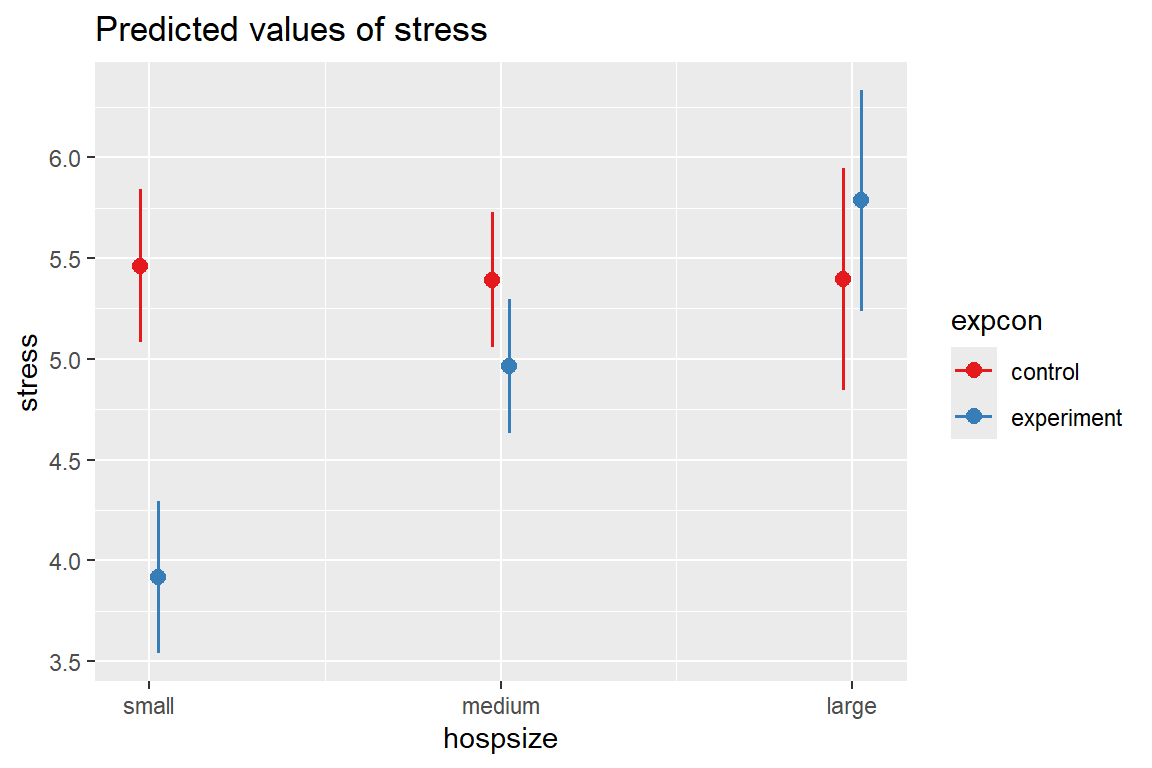
sjPlot::plot_model(fit_lmer_final,
type = "pred",
terms = c("hospsize",
"expcon")) +
labs(title = "Multilevel Modeling of Hospital Nurse Stress Intervention",
subtitle = "Error bars display 95% Confidene Intervals",
x = "Hospital Size",
y = "Estimated Marginal Mean\nNorse's Stress Score",
color = "Condition") +
theme_bw()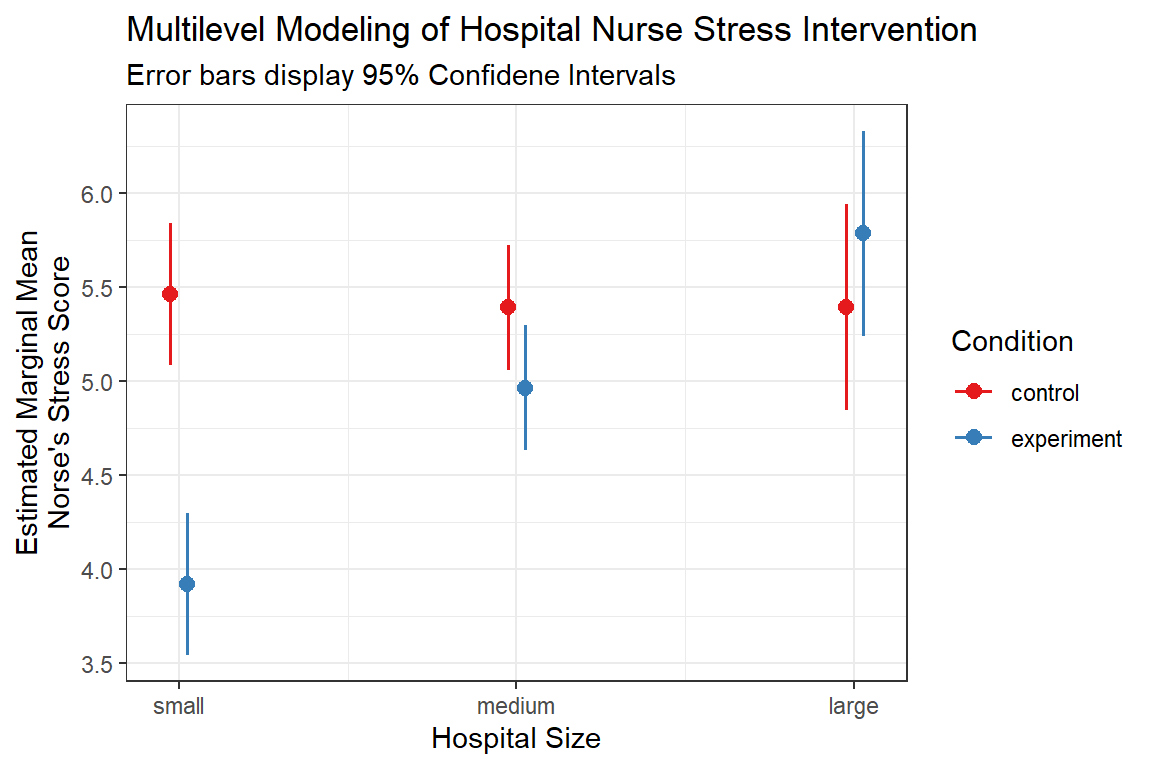
6.10.5.3 Using effects::Effect() and ggplot
Get Estimated Marginal Means - default ‘nice’ predictor values:
Focal predictors: All combinations of…
expconcategorical, both levelscontrolandexperiment
hospsizecategorical, all three levelssmall,medium,large
Always followed by:
fitestimated marginal meansestandard error for the marginal meanlowerlower end of the 95% confidence interval around the estimated marginal meanupperupper end of the 95% confidence interval around the estimated marginal mean
      expcon hospsize      fit        se    lower    upper
1    control    small 5.394485 0.1814379 5.038438 5.750532
2 experiment    small 3.849007 0.1808593 3.494096 4.203919
3    control   medium 5.324360 0.1572391 5.015800 5.632920
4 experiment   medium 4.897002 0.1567719 4.589358 5.204645
5    control    large 5.326344 0.2726473 4.791311 5.861377
6 experiment large 5.718468 0.2717250 5.185245 6.251691 expcon hospsize fit se lower upper
1 control small 5.394485 0.1814379 5.038438 5.750532
2 experiment small 3.849007 0.1808593 3.494096 4.203919
3 control medium 5.324360 0.1572391 5.015800 5.632920
4 experiment medium 4.897002 0.1567719 4.589358 5.204645
5 control large 5.326344 0.2726473 4.791311 5.861377
6 experiment large 5.718468 0.2717250 5.185245 6.251691effects::Effect(focal.predictors = c("expcon", "hospsize"),
mod = fit_lmer_final) %>%
data.frame() %>%
ggplot() +
aes(x = hospsize,
y = fit,
group = expcon,
shape = expcon,
color = expcon) +
geom_errorbar(aes(ymin = fit - se, # mean plus/minus one Std Error
ymax = fit + se),
width = .4,
position = position_dodge(width = .2)) +
geom_errorbar(aes(ymin = lower, # 95% CIs
ymax = upper),
width = .2,
position = position_dodge(width = .2)) +
geom_line(aes(linetype = expcon),
position = position_dodge(width = .2)) +
geom_point(size = 4,
position = position_dodge(width = .2)) +
theme_bw() +
labs(x = "Hospital Size",
y = "Estimated Marginal Mean, Stress",
shape = "Condition",
color = "Condition",
linetype = "Condition") +
theme(legend.key.width = unit(2, "cm"),
legend.background = element_rect(color = "black"),
legend.position = c(1, 0),
legend.justification = c(1.1, -0.1))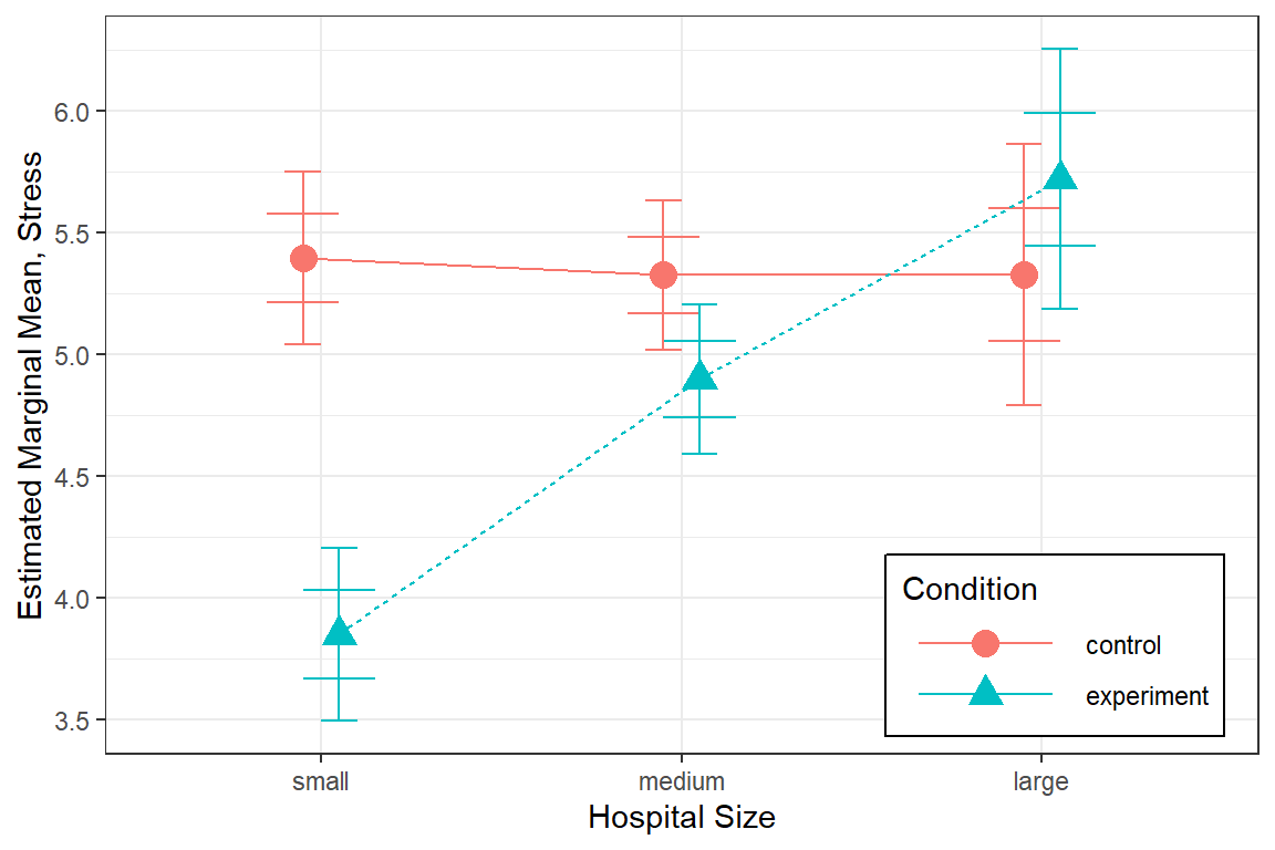
This plot illustrates the estimated marginal means among male (gender’s reference category) nurses at the overall mean age (43.01 years), with the mean level experience (17.06 years), since thoes variables were not included as focal.predictors in the effects::Effect() function. Different values for those predictors would yield the exact sample plot, shifted as a whole either up or down.
6.11 Interpretation
There is evidence this intervention lowered stress among nurses working in small hospitals and to a smaller degree in medium sized hospitals. The intervention did not exhibit an effect in large hospitals.
6.11.1 Strength
This analysis was able to incorporated all three levels of clustering while additionally controlling for many co0-variates, both categorical (nurse gender and ward type) and continuous (nurse age and experience in years). Also heterogeneity was accounted for in terms of the intervention’s effect at various hospitals. This would NOT be possible via any ANOVA type analysis.
6.11.2 Weakness
The approach presented by Hox, Moerbeek, and Van de Schoot (2017) and shown above involved mean-centering categorical variables. This would only be appropriate for a factor with more than two levels if its effect on the outcome was linear. Also, as the mean-centered variables are treated as continuous variables, post hoc tests are increasingly difficult. That is why I did that in the final model.
6.12 Reproduction of Table 2.5
Hox, Moerbeek, and Van de Schoot (2017) presents a table on page 23 comparing various models. Note, that table includes models only fit via maximum likelihood, not REML. Also, the model \(M_3\): with cross-level interaction is slightly different for an unknown reason.
apaSupp::tab_lmers(list("M0" = fit_lmer_0_ml,
                        "M1" = fit_lmer_1d_ml,
                        "M2" = fit_lmer_2_ml,
                        "M3" = fit_lmer_3_ml),
                   narrow = TRUE,
                   caption = "Hox Table 2.5: Models for stress in hospitals and wards")
| M0 | M1 | M2 | M3 | ||||
|---|---|---|---|---|---|---|---|---|
Variable | b | (SE) | b | (SE) | b | (SE) | b | (SE) |
(Intercept) | 5.00 | (0.11) *** | 5.40 | (0.12) *** | 5.39 | (0.11) *** | 5.39 | (0.11) *** |
expconNG | -0.70 | (0.12) *** | -0.70 | (0.18) *** | -0.72 | (0.11) *** | ||
age | 0.02 | (0.00) *** | 0.02 | (0.00) *** | 0.02 | (0.00) *** | ||
gender | -0.45 | (0.03) *** | -0.46 | (0.03) *** | -0.46 | (0.03) *** | ||
experien | -0.06 | (0.00) *** | -0.06 | (0.00) *** | -0.06 | (0.00) *** | ||
wardtype | ||||||||
general care | — | — | — | — | — | — | ||
special care | 0.05 | (0.12) | 0.05 | (0.07) | 0.05 | (0.07) | ||
hospsizeNG | 0.46 | (0.12) ** | 0.46 | (0.12) ** | 0.46 | (0.12) ** | ||
expconNG * hospsizeNG | 1.00 | (0.16) *** | ||||||
ward:hospital.var__(Intercept) | 0.49 | 0.33 | ||||||
hospital.var__(Intercept) | 0.16 | 0.10 | 0.15 | 0.15 | ||||
Residual.var__Observation | 0.30 | 0.22 | 0.22 | 0.22 | ||||
ward.hospital.var__(Intercept) | 0.11 | 0.11 | ||||||
hospital.1.var__expconNG | 0.66 | 0.18 | ||||||
AIC | 1,950 | 1,624 | 1,597 | 1,576 | ||||
BIC | 1,970 | 1,673 | 1,651 | 1,635 | ||||
Log-likelihood | -971 | -802 | -788 | -776 | ||||
Note. | ||||||||
* p < .05. ** p < .01. *** p < .001. | ||||||||
Deviance:
c(deviance(fit_lmer_0_ml),
  deviance(fit_lmer_1d_ml),
  deviance(fit_lmer_2_ml),
  deviance(fit_lmer_3_ml)) %>%
  round(1)
[1] 1942.4 1604.4 1575.5 1552.1