22 GLMM, Proportion Outcome: Meta Analysis (Hox ch 6)

See Appendix E of the Joop Hox text.

https://uoepsy.github.io/msmr/2122/lectures/msmr_lec02_LogisticMLM.html#1

https://commresearch.arizona.edu/classes/comm640/640_Book/docs/multilevel-logistic-regression.html

https://stats.stackexchange.com/questions/544937/when-is-it-appropriate-to-set-nagq-0-in-glmer

https://bookdown.org/animestina/phd_july_19/now-for-advanced-logistic-mixed-effects.html

22.1 PREPARATION

22.1.1 Load Packages

library(tidyverse)  
library(haven)
library(psych)        

library(lme4) 
library(optimx)

library(emmeans)     
library(performance)
library(interactions) 

22.1.2 Background

NESTING * source study id on which multiple conditions were reported (most studies reported on 2 of the 3 modes)

Study Characteristics:

• respisrr type of study reported proportions

• Cr completion rate, # respondents / total sample size

• Rr response rate, sample size was corrected for sampling frame errors

• year 0 = 1947, the oldest year

• saliency saliency of the questionnaire, 0 = not at all, 1 = somewhat, 2 = highly

Condition Characteristics:

• mode dta collection method, 3-levels: Face-to-face, Telephone, or Mail

• tel dummy code for mode = Telephone

• mail dummy code for mode = Mail

• response either the completion rate or response rate

• denom number of respondents approached

22.1.3 Read in the data

df_raw <- haven::read_sav("data/metaresp.sav") %>% 
  haven::as_factor() %>% 
  haven::zap_label() %>% 
  haven::zap_formats() %>% 
  haven::zap_widths() 

tibble::glimpse(df_raw)

Rows: 105
Columns: 14
$ source   <dbl> 1, 1, 1, 2, 2, 2, 3, 3, 4, 4, 5, 5, 6, 6, 7, 7, 8, 8, 9, 9, 9…
$ mode     <fct> ftf, tel, mail, ftf, tel, mail, ftf, mail, ftf, tel, ftf, tel…
$ cr       <dbl> 0.60, 0.64, 0.49, NA, NA, NA, 0.69, 0.72, 0.80, 0.82, 0.32, 0…
$ rr       <dbl> NA, NA, NA, 0.60, 0.52, 0.60, 0.71, 0.73, 0.88, 0.86, 0.36, 0…
$ ftfdum   <fct> ftf condition, not ftf, not ftf, ftf condition, not ftf, not …
$ teldum   <fct> not telephone, telephone condition, not telephone, not teleph…
$ maildum  <fct> notmail, notmail, mail condition, notmail, notmail, mail cond…
$ year     <dbl> 25, 25, 25, 35, 35, 35, 34, 34, 35, 35, 13, 13, 16, 16, 22, 2…
$ saliency <fct> some, some, some, not, not, not, high, high, some, some, not,…
$ denomtot <dbl> 267, 159, 320, NA, NA, NA, 125, 118, 296, 374, 306, 374, 481,…
$ denomcor <dbl> NA, NA, NA, 220, 229, 893, 121, 116, 269, 357, 272, 323, NA, …
$ response <dbl> 0.60, 0.64, 0.49, 0.60, 0.52, 0.60, 0.71, 0.73, 0.88, 0.86, 0…
$ denom    <dbl> 267, 159, 320, 220, 229, 893, 121, 116, 269, 357, 272, 323, 4…
$ respisrr <fct> cr, cr, cr, rr, rr, rr, rr, rr, rr, rr, rr, rr, cr, cr, cr, c…

22.1.4 Long Format

One line per mode per source

df_long <- df_raw %>% 
  dplyr::rename_all(tolower) %>% 
  dplyr::mutate_if(is.factor, ~forcats::fct_relabel(.x, stringr::str_to_title)) %>% 
  dplyr::mutate(res  = round(response*denom, 0)) %>% 
  dplyr::mutate(tel  = as.numeric(mode == "Tel"))%>% 
  dplyr::mutate(mail = as.numeric(mode == "Mail")) %>% 
  dplyr::mutate(yr = year + 1947) %>% 
  dplyr::mutate(yr47 = year) %>% 
  dplyr::mutate(yr77 = year - 30) %>% 
  dplyr::select(source, 
                yr, yr47, yr77,
                saliency,
                mode, tel, mail,
                respisrr,
                response, res, denom)

tibble::glimpse(df_long)

Rows: 105
Columns: 12
$ source   <dbl> 1, 1, 1, 2, 2, 2, 3, 3, 4, 4, 5, 5, 6, 6, 7, 7, 8, 8, 9, 9, 9…
$ yr       <dbl> 1972, 1972, 1972, 1982, 1982, 1982, 1981, 1981, 1982, 1982, 1…
$ yr47     <dbl> 25, 25, 25, 35, 35, 35, 34, 34, 35, 35, 13, 13, 16, 16, 22, 2…
$ yr77     <dbl> -5, -5, -5, 5, 5, 5, 4, 4, 5, 5, -17, -17, -14, -14, -8, -8, …
$ saliency <fct> Some, Some, Some, Not, Not, Not, High, High, Some, Some, Not,…
$ mode     <fct> Ftf, Tel, Mail, Ftf, Tel, Mail, Ftf, Mail, Ftf, Tel, Ftf, Tel…
$ tel      <dbl> 0, 1, 0, 0, 1, 0, 0, 0, 0, 1, 0, 1, 0, 0, 0, 1, 0, 1, 0, 1, 0…
$ mail     <dbl> 0, 0, 1, 0, 0, 1, 0, 1, 0, 0, 0, 0, 0, 1, 0, 0, 0, 0, 0, 0, 1…
$ respisrr <fct> Cr, Cr, Cr, Rr, Rr, Rr, Rr, Rr, Rr, Rr, Rr, Rr, Cr, Cr, Cr, C…
$ response <dbl> 0.60, 0.64, 0.49, 0.60, 0.52, 0.60, 0.71, 0.73, 0.88, 0.86, 0…
$ res      <dbl> 160, 102, 157, 132, 119, 536, 86, 85, 237, 307, 98, 71, 462, …
$ denom    <dbl> 267, 159, 320, 220, 229, 893, 121, 116, 269, 357, 272, 323, 4…

df_long %>% 
  dplyr::select(source, respisrr, mode, tel, mail, yr, saliency, response, denom, res) %>% 
  psych::headTail(top = 10) %>% 
  flextable::flextable() %>% 
  apaSupp::theme_apa(caption = "Meta Data for Response Rate, Long Format")

Table 22.1
Meta Data for Response Rate, Long Format

source	respisrr	mode	tel	mail	yr	saliency	response	denom	res
1	Cr	Ftf	0	0	1972	Some	0.6	267	160
1	Cr	Tel	1	0	1972	Some	0.64	159	102
1	Cr	Mail	0	1	1972	Some	0.49	320	157
2	Rr	Ftf	0	0	1982	Not	0.6	220	132
2	Rr	Tel	1	0	1982	Not	0.52	229	119
2	Rr	Mail	0	1	1982	Not	0.6	893	536
3	Rr	Ftf	0	0	1981	High	0.71	121	86
3	Rr	Mail	0	1	1981	High	0.73	116	85
4	Rr	Ftf	0	0	1982	Some	0.88	269	237
4	Rr	Tel	1	0	1982	Some	0.86	357	307
...			...	...	...		...	...	...
77	Rr	Mail	0	1	1992	Some	0.75	92	69
78	Rr	Ftf	0	0	1992	Some	0.51	476	243
78	Rr	Tel	1	0	1992	Some	0.66	406	268
78	Rr	Mail	0	1	1992	Some	0.67	372	249

22.1.5 Wide Format

One line per source

df_wide <- df_long %>% 
  dplyr::group_by(source) %>% 
  dplyr::mutate(n_modes = n()) %>% 
  dplyr::mutate(respisrr = dplyr::first(respisrr)) %>% 
  dplyr::ungroup() %>% 
  dplyr::select(source, n_modes, yr, yr47, yr77, respisrr, saliency, mode, response) %>% 
  tidyr::pivot_wider(names_from = mode,
                     names_prefix = "resp_",
                     values_from = response)

tibble::glimpse(df_wide)

Rows: 48
Columns: 10
$ source    <dbl> 1, 2, 3, 4, 5, 6, 7, 8, 9, 10, 11, 12, 14, 16, 17, 18, 19, 2…
$ n_modes   <int> 3, 3, 2, 2, 2, 2, 2, 2, 3, 2, 2, 2, 3, 3, 3, 2, 2, 2, 2, 3, …
$ yr        <dbl> 1972, 1982, 1981, 1982, 1960, 1963, 1969, 1969, 1984, 1947, …
$ yr47      <dbl> 25, 35, 34, 35, 13, 16, 22, 22, 37, 0, 31, 31, 31, 20, 20, 2…
$ yr77      <dbl> -5, 5, 4, 5, -17, -14, -8, -8, 7, -30, 1, 1, 1, -10, -10, -6…
$ respisrr  <fct> Cr, Rr, Rr, Rr, Rr, Cr, Cr, Cr, Rr, Cr, Rr, Rr, Rr, Rr, Rr, …
$ saliency  <fct> Some, Not, High, Some, Not, Some, High, High, Some, High, So…
$ resp_Ftf  <dbl> 0.60, 0.60, 0.71, 0.88, 0.36, 0.96, 0.64, 0.68, 0.71, 0.97, …
$ resp_Tel  <dbl> 0.64, 0.52, NA, 0.86, 0.22, NA, 0.72, 0.57, 0.73, NA, 0.59, …
$ resp_Mail <dbl> 0.49, 0.60, 0.73, NA, NA, 0.92, NA, NA, 0.66, 0.82, NA, NA, …

df_wide %>%  
  dplyr::select(-yr47, -yr77) %>% 
  psych::headTail(top = 10) %>% 
  flextable::flextable() %>% 
  apaSupp::theme_apa(caption = "Meta Data for Response Rate, Wide Format")

Table 22.2
Meta Data for Response Rate, Wide Format

source	n_modes	yr	respisrr	saliency	resp_Ftf	resp_Tel	resp_Mail
1	3	1972	Cr	Some	0.6	0.64	0.49
2	3	1982	Rr	Not	0.6	0.52	0.6
3	2	1981	Rr	High	0.71		0.73
4	2	1982	Rr	Some	0.88	0.86
5	2	1960	Rr	Not	0.36	0.22
6	2	1963	Cr	Some	0.96		0.92
7	2	1969	Cr	High	0.64	0.72
8	2	1969	Cr	High	0.68	0.57
9	3	1984	Rr	Some	0.71	0.73	0.66
10	2	1947	Cr	High	0.97		0.82
...	...	...			...	...	...
75	2	1987	Rr	Some	0.79	0.86
76	2	1983	Cr	Not	0.64	0.54
77	3	1992	Rr	Some	0.54	0.64	0.75
78	3	1992	Rr	Some	0.51	0.66	0.67

22.2 EXPLORATORY DATA ANLAYSIS

22.2.1 Sample Size

n = 105 modes/sources

nrow(df_long)

[1] 105

n = 48 sources

nrow(df_wide)

[1] 48

22.2.2 Missing Data - None!

df_long %>% 
  VIM::aggr(numbers = TRUE,   # shows the number to the far right
            prop = FALSE)     # shows counts instead of proportions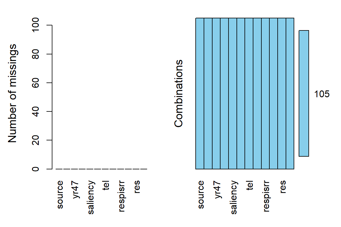

22.2.3 Descriptive Summary

df_wide %>% 
  dplyr::select(n_modes,
                yr,
                resp_Ftf,
                resp_Tel,
                resp_Mail) %>% 
  apaSupp::tab_desc(caption="Descriptive Summary of Sources")

Table 22.3
Descriptive Summary of Sources

	NA	M	SD	min	Q1	Mdn	Q3	max
n_modes	0	2.19	0.53	1.00	2.00	2.00	2.25	3.00
yr	0	1,976.06	9.77	1,947.00	1,969.00	1,978.00	1,983.00	1,992.00
resp_Ftf	8	0.75	0.14	0.36	0.65	0.73	0.87	0.99
resp_Tel	11	0.70	0.16	0.22	0.59	0.73	0.81	0.99
resp_Mail	20	0.65	0.18	0.19	0.63	0.69	0.75	0.95
Note. N = 48. NA = not available or missing; Mdn = median; Q1 = 25th percentile; Q3 = 75th percentile.

df_long %>% 
  dplyr::select(mode,
                yr, saliency,
                respisrr,
                response, res, denom) %>% 
  apaSupp::tab1(split = "mode")

Table 22.4
Summary of Variables

	Total N = 105	Ftf n = 40 (38.1%)	Tel n = 37 (35.2%)	Mail n = 28 (26.7%)	p-value
yr	1,976.74 (9.60)	1,976.73 (10.35)	1,977.68 (8.64)	1,975.54 (9.88)	.662
saliency					.683
Not	19 (18.1%)	6 (15.0%)	9 (24.3%)	4 (14.3%)
Some	60 (57.1%)	22 (55.0%)	20 (54.1%)	18 (64.3%)
High	26 (24.8%)	12 (30.0%)	8 (21.6%)	6 (21.4%)
respisrr					.932
Cr	39 (37.1%)	14 (35.0%)	14 (37.8%)	11 (39.3%)
Rr	66 (62.9%)	26 (65.0%)	23 (62.2%)	17 (60.7%)
response	0.71 (0.16)	0.75 (0.14)	0.70 (0.16)	0.65 (0.18)	.068
res	768.32 (2,095.35)	1,216.85 (3,213.75)	566.76 (1,016.13)	393.93 (342.48)	.198
denom	1,003.32 (2,222.26)	1,458.15 (3,365.10)	772.97 (1,163.73)	657.96 (597.34)	.327
Note. Continuous variables are summarized with means (SD) and significant group differences assessed via independent one-way analysis of vaiance (ANOVA). Categorical variables are summarized with counts (%) and significant group differences assessed via Chi-squared tests for independence.
* p < .05. ** p < .01. *** p < .001.

df_wide %>% 
  apaSupp::spicy_histos(yr)

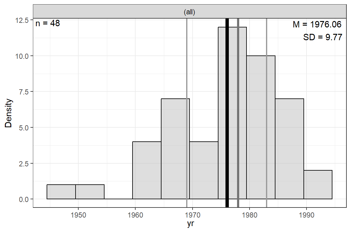
Figure 22.1
Distribution of Source Year (0 for 1947)

22.3 MULTILEVEL MODELING

22.3.1 Base Model

22.3.1.1 PQL

fit_glmer_0 <- lme4::glmer(cbind(res, denom - res) ~ respisrr + (1|source),
                              data = df_long,
                              family = binomial,
                              nAGQ = 0)

summary(fit_glmer_0)

Generalized linear mixed model fit by maximum likelihood (Adaptive
  Gauss-Hermite Quadrature, nAGQ = 0) [glmerMod]
 Family: binomial  ( logit )
Formula: cbind(res, denom - res) ~ respisrr + (1 | source)
   Data: df_long

      AIC       BIC    logLik -2*log(L)  df.resid 
     2236      2244     -1115      2230       102 

Scaled residuals: 
    Min      1Q  Median      3Q     Max 
-11.973  -1.893   0.062   1.881  11.112 

Random effects:
 Groups Name        Variance Std.Dev.
 source (Intercept) 0.92     0.959   
Number of obs: 105, groups:  source, 48

Fixed effects:
            Estimate Std. Error z value Pr(>|z|)    
(Intercept)   0.5907     0.1440     4.1  4.1e-05 ***
respisrrRr    0.7012     0.0579    12.1  < 2e-16 ***
---
Signif. codes:  0 '***' 0.001 '**' 0.01 '*' 0.05 '.' 0.1 ' ' 1

Correlation of Fixed Effects:
           (Intr)
respisrrRr -0.243

22.3.1.2 Laplace

fit_glmer_1 <- lme4::glmer(cbind(res, denom - res) ~ respisrr + (1|source),
                              data = df_long,
                              family = binomial)

summary(fit_glmer_1)

Generalized linear mixed model fit by maximum likelihood (Laplace
  Approximation) [glmerMod]
 Family: binomial  ( logit )
Formula: cbind(res, denom - res) ~ respisrr + (1 | source)
   Data: df_long

      AIC       BIC    logLik -2*log(L)  df.resid 
     2236      2244     -1115      2230       102 

Scaled residuals: 
    Min      1Q  Median      3Q     Max 
-11.973  -1.893   0.062   1.881  11.111 

Random effects:
 Groups Name        Variance Std.Dev.
 source (Intercept) 0.92     0.959   
Number of obs: 105, groups:  source, 48

Fixed effects:
            Estimate Std. Error z value Pr(>|z|)    
(Intercept)   0.5948     0.1440    4.13  3.6e-05 ***
respisrrRr    0.7012     0.0582   12.06  < 2e-16 ***
---
Signif. codes:  0 '***' 0.001 '**' 0.01 '*' 0.05 '.' 0.1 ' ' 1

Correlation of Fixed Effects:
           (Intr)
respisrrRr -0.241

22.3.1.3 Compare

apaSupp::tab_lmers(list("PQL" = fit_glmer_0,
                        "Laplace" = fit_glmer_1))

Table 22.5
Compare MLM Models

	PQL			Laplace
Variable	b	(SE)	p	b	(SE)	p
(Intercept)	0.59	(0.14)	< .001***	0.59	(0.14)	< .001***
respisrr
Cr	—	—		—	—
Rr	0.70	(0.06)	< .001***	0.70	(0.06)	< .001***
source.var__(Intercept)	0.92			0.92
AIC	2,236			2,236
BIC	2,244			2,244
Log-likelihood	-1,115			-1,115
Note.
* p < .05. ** p < .01. *** p < .001.

22.3.2 Main Effect of Model

22.3.2.1 Random Intercepts

fit_glmer_2 <- lme4::glmer(cbind(res, denom - res) ~ respisrr + mode + (1|source),
                              data = df_long,
                              family = binomial)

summary(fit_glmer_2)

Generalized linear mixed model fit by maximum likelihood (Laplace
  Approximation) [glmerMod]
 Family: binomial  ( logit )
Formula: cbind(res, denom - res) ~ respisrr + mode + (1 | source)
   Data: df_long

      AIC       BIC    logLik -2*log(L)  df.resid 
     1939      1952      -964      1929       100 

Scaled residuals: 
    Min      1Q  Median      3Q     Max 
-10.278  -1.757   0.062   1.811   8.039 

Random effects:
 Groups Name        Variance Std.Dev.
 source (Intercept) 0.849    0.921   
Number of obs: 105, groups:  source, 48

Fixed effects:
            Estimate Std. Error z value Pr(>|z|)    
(Intercept)   0.9045     0.1405    6.44  1.2e-10 ***
respisrrRr    0.5274     0.0608    8.68  < 2e-16 ***
modeTel      -0.1600     0.0211   -7.59  3.2e-14 ***
modeMail     -0.4875     0.0282  -17.27  < 2e-16 ***
---
Signif. codes:  0 '***' 0.001 '**' 0.01 '*' 0.05 '.' 0.1 ' ' 1

Correlation of Fixed Effects:
           (Intr) rspsrR modeTl
respisrrRr -0.280              
modeTel    -0.142  0.297       
modeMail   -0.118  0.135  0.335

22.3.2.2 Add Random Slopes

fit_glmer_3 <- lme4::glmer(cbind(res, denom - res) ~ respisrr + mode + 
                                (1|source) + (0 + tel|source) + (0+ mail|source),
                              data = df_long,
                              family = binomial)

summary(fit_glmer_3)

Generalized linear mixed model fit by maximum likelihood (Laplace
  Approximation) [glmerMod]
 Family: binomial  ( logit )
Formula: cbind(res, denom - res) ~ respisrr + mode + (1 | source) + (0 +  
    tel | source) + (0 + mail | source)
   Data: df_long

      AIC       BIC    logLik -2*log(L)  df.resid 
     1150      1169      -568      1136        98 

Scaled residuals: 
    Min      1Q  Median      3Q     Max 
-1.2636 -0.1418  0.0099  0.1968  1.2858 

Random effects:
 Groups   Name        Variance Std.Dev.
 source   (Intercept) 0.766    0.875   
 source.1 tel         0.241    0.491   
 source.2 mail        0.443    0.666   
Number of obs: 105, groups:  source, 48

Fixed effects:
            Estimate Std. Error z value Pr(>|z|)    
(Intercept)   1.1429     0.2030    5.63  1.8e-08 ***
respisrrRr    0.1886     0.2346    0.80  0.42156    
modeTel      -0.1756     0.0926   -1.90  0.05796 .  
modeMail     -0.5103     0.1444   -3.53  0.00041 ***
---
Signif. codes:  0 '***' 0.001 '**' 0.01 '*' 0.05 '.' 0.1 ' ' 1

Correlation of Fixed Effects:
           (Intr) rspsrR modeTl
respisrrRr -0.755              
modeTel    -0.138  0.103       
modeMail   -0.174  0.120  0.130

22.3.2.3 Compare

apaSupp::tab_lmers(list("RI" = fit_glmer_2,
                        "RIAS" = fit_glmer_3))

Table 22.6
Compare MLM Models

	RI			RIAS
Variable	b	(SE)	p	b	(SE)	p
(Intercept)	0.90	(0.14)	< .001***	1.14	(0.20)	< .001***
respisrr
Cr	—	—		—	—
Rr	0.53	(0.06)	< .001***	0.19	(0.23)	.422
mode
Ftf	—	—		—	—
Tel	-0.16	(0.02)	< .001***	-0.18	(0.09)	.058
Mail	-0.49	(0.03)	< .001***	-0.51	(0.14)	< .001***
source.var__(Intercept)	0.85			0.77
source.1.var__tel				0.24
source.2.var__mail				0.44
AIC	1,939			1,150
BIC	1,952			1,169
Log-likelihood	-964			-568
Note.
* p < .05. ** p < .01. *** p < .001.

apaSupp::tab_lmer_fits(list("RI" = fit_glmer_2,
                            "RIAS" = fit_glmer_3))

Table 22.7
Comparison of MLM Performane Metrics

Model	AIC	BIC	RMSE	$R^2$
				Conditional	Marginal
RI	1938.61	1951.88	0.07	.997	.112
RIAS	1150.49	1169.07	0.01	.996	.062
Note. Larger $R^2$ values indicated better performance. Smaller values indicated better performance for Akaike's Information Criteria (AIC), Bayesian information criteria (BIC), and Root Mean Squared Error (RMSE).

anova(fit_glmer_2, fit_glmer_3)

Data: df_long
Models:
fit_glmer_2: cbind(res, denom - res) ~ respisrr + mode + (1 | source)
fit_glmer_3: cbind(res, denom - res) ~ respisrr + mode + (1 | source) + (0 + tel | source) + (0 + mail | source)
            npar  AIC  BIC logLik -2*log(L) Chisq Df Pr(>Chisq)    
fit_glmer_2    5 1939 1952   -964      1929                        
fit_glmer_3    7 1150 1169   -568      1136   792  2     <2e-16 ***
---
Signif. codes:  0 '***' 0.001 '**' 0.01 '*' 0.05 '.' 0.1 ' ' 1

22.3.3 Cross-Level Interaction

Helps for “failed to converge”: https://cran.r-project.org/web/packages/lme4/vignettes/lmerperf.html

fit_glmer_4 <- lme4::glmer(cbind(res, denom - res) ~ respisrr + mode + 
                                saliency + yr77 +
                                (1|source) + (0 + tel|source) + (0+ mail|source),
                              data = df_long,
                              family = binomial,
                              control=glmerControl(optimizer="bobyqa",
                                                   optCtrl=list(maxfun=100000)))

summary(fit_glmer_4)

Generalized linear mixed model fit by maximum likelihood (Laplace
  Approximation) [glmerMod]
 Family: binomial  ( logit )
Formula: cbind(res, denom - res) ~ respisrr + mode + saliency + yr77 +  
    (1 | source) + (0 + tel | source) + (0 + mail | source)
   Data: df_long
Control: glmerControl(optimizer = "bobyqa", optCtrl = list(maxfun = 1e+05))

      AIC       BIC    logLik -2*log(L)  df.resid 
     1138      1164      -559      1118        95 

Scaled residuals: 
    Min      1Q  Median      3Q     Max 
-1.2213 -0.1306  0.0093  0.2001  1.0561 

Random effects:
 Groups   Name        Variance Std.Dev.
 source   (Intercept) 0.516    0.719   
 source.1 tel         0.252    0.502   
 source.2 mail        0.409    0.640   
Number of obs: 105, groups:  source, 48

Fixed effects:
             Estimate Std. Error z value Pr(>|z|)    
(Intercept)    0.3438     0.2841    1.21  0.22622    
respisrrRr     0.2527     0.2130    1.19  0.23531    
modeTel       -0.1558     0.0940   -1.66  0.09740 .  
modeMail      -0.5037     0.1392   -3.62  0.00029 ***
saliencySome   0.6800     0.2963    2.30  0.02172 *  
saliencyHigh   1.3583     0.3320    4.09  4.3e-05 ***
yr77          -0.0230     0.0118   -1.94  0.05249 .  
---
Signif. codes:  0 '***' 0.001 '**' 0.01 '*' 0.05 '.' 0.1 ' ' 1

Correlation of Fixed Effects:
            (Intr) rspsrR modeTl modeMl slncyS slncyH
respisrrRr  -0.437                                   
modeTel     -0.121  0.085                            
modeMail    -0.115  0.102  0.129                     
saliencySom -0.722 -0.111  0.035 -0.003              
saliencyHgh -0.689  0.016  0.058  0.028  0.644       
yr77         0.136 -0.192  0.002  0.054 -0.078  0.051

fit_glmer_5 <- lme4::glmer(cbind(res, denom - res) ~ respisrr + mode + 
                                saliency + mode*yr77 +
                                (1|source) + (0 + tel|source) + (0+ mail|source),
                              data = df_long,
                              family = binomial,
                              control=glmerControl(optimizer="bobyqa",
                                                   optCtrl=list(maxfun=100000)))

summary(fit_glmer_5)

Generalized linear mixed model fit by maximum likelihood (Laplace
  Approximation) [glmerMod]
 Family: binomial  ( logit )
Formula: cbind(res, denom - res) ~ respisrr + mode + saliency + mode *  
    yr77 + (1 | source) + (0 + tel | source) + (0 + mail | source)
   Data: df_long
Control: glmerControl(optimizer = "bobyqa", optCtrl = list(maxfun = 1e+05))

      AIC       BIC    logLik -2*log(L)  df.resid 
     1131      1163      -554      1107        93 

Scaled residuals: 
    Min      1Q  Median      3Q     Max 
-0.8668 -0.1418  0.0197  0.1920  1.0444 

Random effects:
 Groups   Name        Variance Std.Dev.
 source   (Intercept) 0.541    0.736   
 source.1 tel         0.224    0.473   
 source.2 mail        0.321    0.567   
Number of obs: 105, groups:  source, 48

Fixed effects:
              Estimate Std. Error z value Pr(>|z|)    
(Intercept)     0.3505     0.2882    1.22   0.2239    
respisrrRr      0.2629     0.2105    1.25   0.2117    
modeTel        -0.1797     0.0909   -1.98   0.0479 *  
modeMail       -0.4940     0.1263   -3.91  9.2e-05 ***
saliencySome    0.6876     0.3013    2.28   0.0225 *  
saliencyHigh    1.3784     0.3389    4.07  4.8e-05 ***
yr77           -0.0287     0.0122   -2.34   0.0192 *  
modeTel:yr77    0.0209     0.0101    2.06   0.0389 *  
modeMail:yr77   0.0363     0.0134    2.70   0.0069 ** 
---
Signif. codes:  0 '***' 0.001 '**' 0.01 '*' 0.05 '.' 0.1 ' ' 1

Correlation of Fixed Effects:
            (Intr) rspsrR modeTl modeMl slncyS slncyH yr77   mdT:77
respisrrRr  -0.429                                                 
modeTel     -0.128  0.089                                          
modeMail    -0.115  0.098  0.145                                   
saliencySom -0.730 -0.101  0.039  0.002                            
saliencyHgh -0.692  0.019  0.064  0.028  0.646                     
yr77         0.135 -0.193  0.006  0.050 -0.080  0.041              
modeTl:yr77  0.037 -0.011 -0.143 -0.026 -0.024 -0.026 -0.052       
modeMl:yr77  0.018 -0.043 -0.015  0.020  0.038  0.030 -0.160  0.046

22.3.3.1 Compare

apaSupp::tab_lmers(list("Main Effect" = fit_glmer_4,
                        "Intraction" = fit_glmer_5))

Table 22.8
Compare MLM Models

	Main Effect			Intraction
Variable	b	(SE)	p	b	(SE)	p
(Intercept)	0.34	(0.28)	.226	0.35	(0.29)	.224
respisrr
Cr	—	—		—	—
Rr	0.25	(0.21)	.235	0.26	(0.21)	.212
mode
Ftf	—	—		—	—
Tel	-0.16	(0.09)	.097	-0.18	(0.09)	.048*
Mail	-0.50	(0.14)	< .001***	-0.49	(0.13)	< .001***
saliency
Not	—	—		—	—
Some	0.68	(0.30)	.022*	0.69	(0.30)	.022*
High	1.36	(0.33)	< .001***	1.38	(0.34)	< .001***
yr77	-0.02	(0.01)	.052	-0.03	(0.01)	.019*
mode * yr77
Tel * yr77				0.02	(0.01)	.039*
Mail * yr77				0.04	(0.01)	.007**
source.var__(Intercept)	0.52			0.54
source.1.var__tel	0.25			0.22
source.2.var__mail	0.41			0.32
AIC	1,138			1,131
BIC	1,164			1,163
Log-likelihood	-559			-554
Note.
* p < .05. ** p < .01. *** p < .001.

apaSupp::tab_lmer_fits(list("Main Effect" = fit_glmer_4,
                            "Intraction" = fit_glmer_5))

Table 22.9
Comparison of MLM Performane Metrics

Model	AIC	BIC	RMSE	$R^2$
				Conditional	Marginal
Main Effect	1137.61	1164.15	0.01	.996	.362
Intraction	1131.18	1163.03	0.01	.996	.350
Note. Larger $R^2$ values indicated better performance. Smaller values indicated better performance for Akaike's Information Criteria (AIC), Bayesian information criteria (BIC), and Root Mean Squared Error (RMSE).

anova(fit_glmer_4, fit_glmer_5)

Data: df_long
Models:
fit_glmer_4: cbind(res, denom - res) ~ respisrr + mode + saliency + yr77 + (1 | source) + (0 + tel | source) + (0 + mail | source)
fit_glmer_5: cbind(res, denom - res) ~ respisrr + mode + saliency + mode * yr77 + (1 | source) + (0 + tel | source) + (0 + mail | source)
            npar  AIC  BIC logLik -2*log(L) Chisq Df Pr(>Chisq)   
fit_glmer_4   10 1138 1164   -559      1118                       
fit_glmer_5   12 1131 1163   -554      1107  10.4  2     0.0054 **
---
Signif. codes:  0 '***' 0.001 '**' 0.01 '*' 0.05 '.' 0.1 ' ' 1

22.3.4 Predicted Probabilities

22.3.4.1 At the Mean Year (1977)

fit_glmer_5 %>% 
  emmeans::emmeans(~ mode*saliency,
                   at = list(yr77 = 0,
                             saliency = c("Not", "High")),
                   type = "response")

 mode saliency  prob     SE  df asymp.LCL asymp.UCL
 Ftf  Not      0.618 0.0616 Inf     0.493     0.730
 Tel  Not      0.575 0.0653 Inf     0.445     0.695
 Mail Not      0.497 0.0699 Inf     0.363     0.631
 Ftf  High     0.865 0.0258 Inf     0.806     0.908
 Tel  High     0.843 0.0314 Inf     0.771     0.895
 Mail High     0.797 0.0402 Inf     0.707     0.864

Results are averaged over the levels of: respisrr 
Confidence level used: 0.95 
Intervals are back-transformed from the logit scale 

22.3.4.2 Each Mode Across Years

fit_glmer_5 %>% 
  emmeans::emmeans(~ mode*yr77,
                   at = list(yr77 = c(1950-1977, 
                                      1977-1977, 
                                      1990-1977)),
                   type = "response")

 mode yr77  prob     SE  df asymp.LCL asymp.UCL
 Ftf   -27 0.875 0.0372 Inf     0.782     0.932
 Tel   -27 0.769 0.0777 Inf     0.585     0.887
 Mail  -27 0.616 0.1080 Inf     0.396     0.797
 Ftf     0 0.763 0.0232 Inf     0.715     0.806
 Tel     0 0.729 0.0291 Inf     0.669     0.782
 Mail    0 0.663 0.0371 Inf     0.587     0.731
 Ftf    13 0.689 0.0463 Inf     0.592     0.772
 Tel    13 0.709 0.0526 Inf     0.596     0.801
 Mail   13 0.685 0.0629 Inf     0.551     0.794

Results are averaged over the levels of: respisrr, saliency 
Confidence level used: 0.95 
Intervals are back-transformed from the logit scale 

fit_glmer_5 %>% 
  emmeans::emmeans(~ mode*yr77,
                   at = list(yr77 = c(1950-1977, 
                                      1977-1977, 
                                      1990-1977)),
                   type = "response") %>% 
  data.frame() %>% 
  dplyr::mutate(year = as.character(1977 + yr77)) %>% 
  dplyr::mutate(mode = mode %>% 
                  forcats::fct_recode("Face-to-Face" = "Ftf",
                                      "Telephone" = "Tel",
                                      "Mail" = "Mail")) %>% 
  dplyr::mutate(across(c(prob, asymp.LCL, asymp.UCL),
                       ~apaSupp::p_num(.x, stars = FALSE))) %>% 
  dplyr::mutate(cell = glue::glue("{prob} [{asymp.LCL}, {asymp.UCL}]")) %>% 
  dplyr::select(mode, year, cell) %>% 
  tidyr::pivot_wider(names_from = year,
                     values_from = cell) %>% 
  flextable::flextable() %>% 
  apaSupp::theme_apa(caption = "Predicted Response Rates for Each Mode at Key Years, [95% CI]",
                     general_note = "Predications are for 'some' saliency.")

Table 22.10
Predicted Response Rates for Each Mode at Key Years, [95% CI]

mode	1950	1977	1990
Face-to-Face	.875 [ .782 , .932 ]	.763 [ .715 , .806 ]	.689 [ .592 , .772 ]
Telephone	.769 [ .585 , .887 ]	.729 [ .669 , .782 ]	.709 [ .596 , .801 ]
Mail	.616 [ .396 , .797 ]	.663 [ .587 , .731 ]	.685 [ .551 , .794 ]
Note. Predications are for 'some' saliency.

22.3.4.3 Pairwise Comparisons

fit_glmer_5 %>% 
  emmeans::emmeans(~ mode*saliency|yr77,
                   at = list(saliency = "Some",
                             yr77 = c(1950-1977, 
                                      1977-1977, 
                                      1990-1977)),
                   type = "response") %>% 
  pairs(adjust = "none")

yr77 = -27:
 contrast             odds.ratio    SE  df null z.ratio p.value
 Ftf Some / Tel Some        2.11 0.632 Inf    1   2.480  0.0130
 Ftf Some / Mail Some       4.36 1.660 Inf    1   3.860  <.0001
 Tel Some / Mail Some       2.07 0.973 Inf    1   1.550  0.1210

yr77 = 0:
 contrast             odds.ratio    SE  df null z.ratio p.value
 Ftf Some / Tel Some        1.20 0.109 Inf    1   1.980  0.0480
 Ftf Some / Mail Some       1.64 0.207 Inf    1   3.910  <.0001
 Tel Some / Mail Some       1.37 0.198 Inf    1   2.170  0.0300

yr77 = 13:
 contrast             odds.ratio    SE  df null z.ratio p.value
 Ftf Some / Tel Some        0.91 0.136 Inf    1  -0.620  0.5360
 Ftf Some / Mail Some       1.02 0.222 Inf    1   0.100  0.9170
 Tel Some / Mail Some       1.12 0.287 Inf    1   0.450  0.6530

Results are averaged over the levels of: respisrr 
Tests are performed on the log odds ratio scale 

fit_glmer_5 %>% 
  emmeans::emmeans(~ mode*saliency|yr77,
                   at = list(saliency = "Some",
                             yr77 = c(1950-1977, 
                                      1977-1977, 
                                      1990-1977)),
                   type = "response") %>% 
  pairs(adjust = "none") %>% 
  data.frame() %>% 
  dplyr::mutate(yr77 = as.numeric(as.character(yr77))) %>% 
  dplyr::mutate(year = as.character(1977 + yr77)) %>% 
  dplyr::mutate(contrast = contrast %>% 
                  forcats::fct_recode("Face-to-Face vs. Telephone" = "Ftf Some / Tel Some",
                                      "Face-to-Face vs. Mail" = "Ftf Some / Mail Some",
                                      "Telephone vs. Mail" = "Tel Some / Mail Some")) %>% 
  dplyr::mutate(p.adj = p.adjust(p.value, method = "fdr")) %>% 
  dplyr::mutate(across(c(p.value, p.adj), apaSupp::p_num)) %>% 
  dplyr::select(Year = year, 
                "Comparing Modes" = contrast, 
                OR = odds.ratio,
                p_Unadj = p.value,
                p_Adj = p.adj) %>% 
  flextable::as_grouped_data(groups = "Year") %>% 
  flextable::flextable() %>% 
  flextable::separate_header() %>% 
  apaSupp::theme_apa(caption = "Pairwise Comparisons Between Survey Mode at Key Years",
                     general_note = "Significance is given both unadjusted (Unadj) and adjusted (Adj) via the method of Benjamini, Hochberg, and Yekutieli to control the false discovery rate (FDR).")

Table 22.11
Pairwise Comparisons Between Survey Mode at Key Years

Year	Comparing Modes	OR	p
			Unadj	Adj
1950
	Face-to-Face vs. Telephone	2.11	.013*	.040*
	Face-to-Face vs. Mail	4.36	< .001***	< .001***
	Telephone vs. Mail	2.07	.121	.181
1977
	Face-to-Face vs. Telephone	1.20	.048*	.086
	Face-to-Face vs. Mail	1.64	< .001***	< .001***
	Telephone vs. Mail	1.37	.030*	.067
1990
	Face-to-Face vs. Telephone	0.91	.536	.689
	Face-to-Face vs. Mail	1.02	.917	.917
	Telephone vs. Mail	1.12	.653	.735
Note. Significance is given both unadjusted (Unadj) and adjusted (Adj) via the method of Benjamini, Hochberg, and Yekutieli to control the false discovery rate (FDR).

22.3.5 Plot

22.3.5.1 Simple

interactions::interact_plot(model = fit_glmer_5,
                            pred = yr77,
                            modx = mode,
                            interval = TRUE,
                            int.width = .685)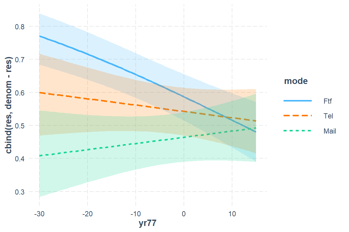

22.3.5.2 Publishable

fit_glmer_5 %>% 
  emmeans::emmeans(~ yr77*mode,
                   at = list(yr77 = seq(from = 1947 - 1977, 
                                        to = 1992 - 1977, 
                                        by = 1)),
                   type = "response",
                   level = .685) %>% 
  data.frame() %>% 
  dplyr::mutate(year = 1977 + yr77) %>% 
  dplyr::mutate(mode = mode %>% 
                  forcats::fct_recode("Face-to-Face" = "Ftf",
                                      "Telephone" = "Tel",
                                      "Mail" = "Mail")) %>% 
  ggplot(aes(x = year,
             y = prob,
             linetype = mode)) +
  # geom_ribbon(aes(ymin = asymp.LCL,
  #                 ymax = asymp.UCL),
  #             alpha= .15) +
  geom_line(linewidth = 1) +
  labs(x = NULL,
       y = "Predicted Response Rate",
       linetype = "Collection Mode") +
  theme_bw() +
  geom_vline(xintercept = c(1950, 1977, 1990),
             linewidth = 3,
             alpha = .2) +
  scale_linetype_manual(values = c("solid", "longdash", "dotted")) +
  theme(legend.position = "inside",
        legend.position.inside = c(.92, 1.0),
        legend.justification = c(1.1, 1.1),
        legend.background = element_rect(color = "black"),
        legend.key.width = unit(1.5, "cm"))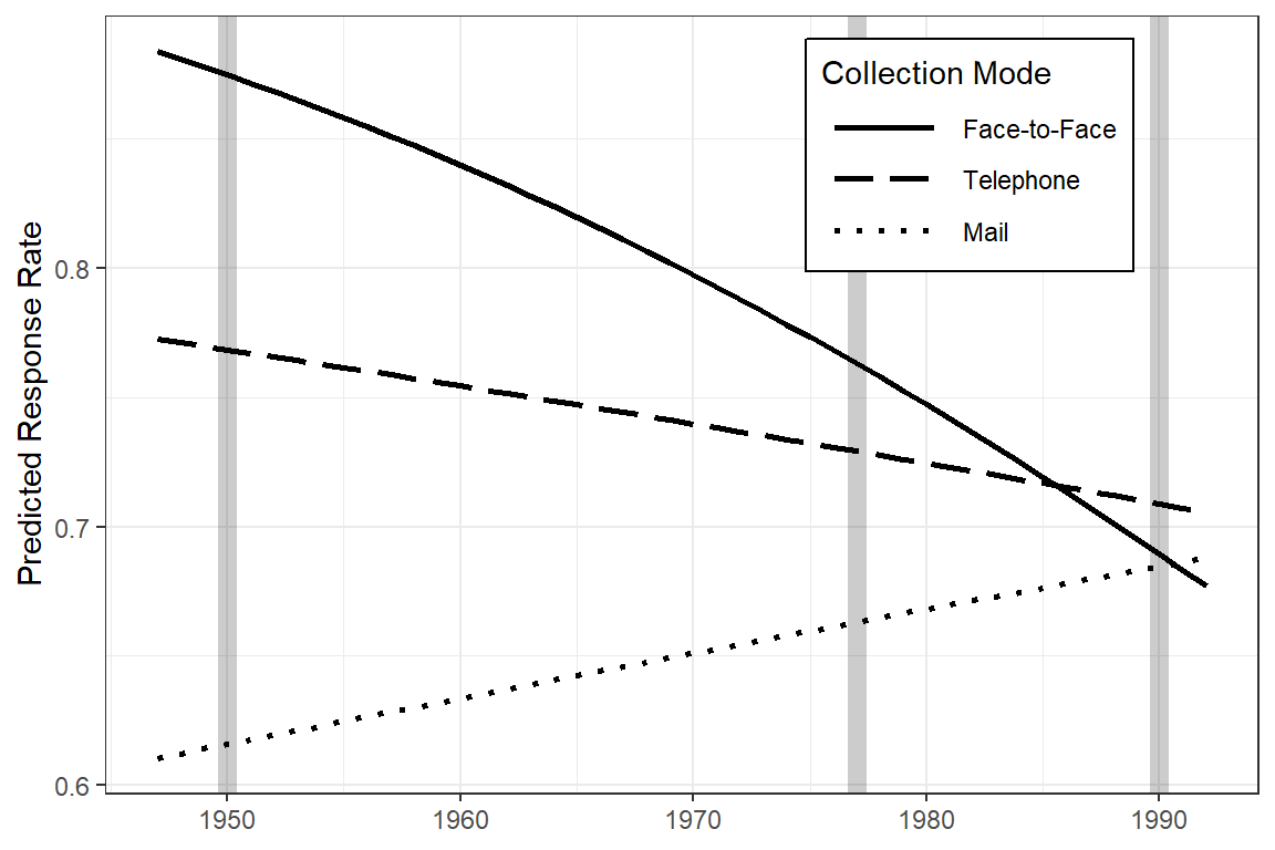

Figure 22.2
Predicted Response Rates Over the Years (Hox figure 6.2 on page 122)

https://glennwilliams.me/r4psych/mixed-effects-models.html#a-note-on-power-effect-sizes-and-pairwise-comparisons