17 GEE, Count Outcome: Epilepsy
17.1 PREPARATION
17.1.1 Load Packages
install.packages("devtools")
devtools::install_github("sarbearschwartz/apaSupp") # updated 10/14/2025
Load/activate these packages
17.1.2 Background
This dataset was used as an example in Chapter 11 of “A Handbook of Statistical Analysis using R” by Brian S. Everitt and Torsten Hothorn. The authors include this data set in their HSAUR package on
CRAN.
The Background
In this clinical trial, 59 patients suffering from epilepsy were randomized to groups receiving either the anti-epileptic drug “Progabide”” or a placebo in addition to standard chemotherapy. The numbers of seizures suffered in each of four, two-week periods were recorded for each patient along with a baseline seizure count for the 8 weeks prior to being randomized to treatment and age.
The Research Question
The main question of interest is whether taking progabide reduced the number of epileptic seizures compared with placebo.
The Data
Indicators
subjectthe patient ID, a factor with levels 1 to 59
periodtreatment period, an ordered factor with levels 1 to 4
Outcome or dependent variable
+
seizure.ratethe number of seizures (2-weeks)Main predictor or independent variable of interest
treatmentthe treatment group, a factor with levels placebo and Progabide
Time-invariant Covariates
agethe age of the patient
basethe number of seizures before the trial (8 weeks)
17.1.3 Read in the data
Problem: The outcome (seizure.rate) were counts over a TWO-week period and we would like to interpret the results in terms of effects on the WEEKLY rate.
- If we divide the values by TWO to get weekly rates, the outcome might be a decimal number
- The Poisson distribution may only be used for whole numbers (not deciamls)
Solution: We need to include an offset term in the model that indicates the LOG DURATION of each period.
- Every observation period is exactly 2 weeks in this experiment
- Create a variable in the original dataset that is equal to the LOG DURATION (
per = log(2)) - To the formula for the
glm()orgee(), add:+ offset(per)
17.1.4 Long Format
df_long <- epilepsy %>%
  dplyr::select(subject, age, treatment, base,
                period, seizure.rate) %>%
  dplyr::mutate(per = log(2)) %>%                  # new variable to use with the offset
dplyr::mutate(base_wk = base/8)'data.frame': 236 obs. of 8 variables:
$ subject : Factor w/ 59 levels "1","2","3","4",..: 1 1 1 1 2 2 2 2 3 3 ...
$ age : int 31 31 31 31 30 30 30 30 25 25 ...
$ treatment : Factor w/ 2 levels "placebo","Progabide": 1 1 1 1 1 1 1 1 1 1 ...
$ base : int 11 11 11 11 11 11 11 11 6 6 ...
$ period : Ord.factor w/ 4 levels "1"<"2"<"3"<"4": 1 2 3 4 1 2 3 4 1 2 ...
$ seizure.rate: int 5 3 3 3 3 5 3 3 2 4 ...
$ per : num 0.693 0.693 0.693 0.693 0.693 ...
$ base_wk : num 1.38 1.38 1.38 1.38 1.38 ...df_long %>%
psych::headTail(, top = 10, bottom = 6) %>%
flextable::flextable() %>%
apaSupp::theme_apa(caption = "Long Form of the Data")subject | age | treatment | base | period | seizure.rate | per | base_wk |
|---|---|---|---|---|---|---|---|
1 | 31 | placebo | 11 | 1 | 5 | 0.69 | 1.38 |
1 | 31 | placebo | 11 | 2 | 3 | 0.69 | 1.38 |
1 | 31 | placebo | 11 | 3 | 3 | 0.69 | 1.38 |
1 | 31 | placebo | 11 | 4 | 3 | 0.69 | 1.38 |
2 | 30 | placebo | 11 | 1 | 3 | 0.69 | 1.38 |
2 | 30 | placebo | 11 | 2 | 5 | 0.69 | 1.38 |
2 | 30 | placebo | 11 | 3 | 3 | 0.69 | 1.38 |
2 | 30 | placebo | 11 | 4 | 3 | 0.69 | 1.38 |
3 | 25 | placebo | 6 | 1 | 2 | 0.69 | 0.75 |
3 | 25 | placebo | 6 | 2 | 4 | 0.69 | 0.75 |
... | ... | ... | ... | ... | |||
58 | 36 | Progabide | 13 | 3 | 0 | 0.69 | 1.62 |
58 | 36 | Progabide | 13 | 4 | 0 | 0.69 | 1.62 |
59 | 37 | Progabide | 12 | 1 | 1 | 0.69 | 1.5 |
59 | 37 | Progabide | 12 | 2 | 4 | 0.69 | 1.5 |
59 | 37 | Progabide | 12 | 3 | 3 | 0.69 | 1.5 |
59 | 37 | Progabide | 12 | 4 | 2 | 0.69 | 1.5 |
17.1.5 Wide Format
df_wide <- df_long %>%
  tidyr::spread(key = period,
                value = seizure.rate,
                sep = "_") %>%
dplyr::arrange(subject)'data.frame': 59 obs. of 10 variables:
$ subject : Factor w/ 59 levels "1","2","3","4",..: 1 2 3 4 5 6 7 8 9 10 ...
$ age : int 31 30 25 36 22 29 31 42 37 28 ...
$ treatment: Factor w/ 2 levels "placebo","Progabide": 1 1 1 1 1 1 1 1 1 1 ...
$ base : int 11 11 6 8 66 27 12 52 23 10 ...
$ per : num 0.693 0.693 0.693 0.693 0.693 ...
$ base_wk : num 1.38 1.38 0.75 1 8.25 ...
$ period_1 : int 5 3 2 4 7 5 6 40 5 14 ...
$ period_2 : int 3 5 4 4 18 2 4 20 6 13 ...
$ period_3 : int 3 3 0 1 9 8 0 23 6 6 ...
$ period_4 : int 3 3 5 4 21 7 2 12 5 0 ...df_wide %>%
psych::headTail(, top = 10, bottom = 6) %>%
flextable::flextable() %>%
apaSupp::theme_apa(caption = "Wide Form of the Data")subject | age | treatment | base | per | base_wk | period_1 | period_2 | period_3 | period_4 |
|---|---|---|---|---|---|---|---|---|---|
1 | 31 | placebo | 11 | 0.69 | 1.38 | 5 | 3 | 3 | 3 |
2 | 30 | placebo | 11 | 0.69 | 1.38 | 3 | 5 | 3 | 3 |
3 | 25 | placebo | 6 | 0.69 | 0.75 | 2 | 4 | 0 | 5 |
4 | 36 | placebo | 8 | 0.69 | 1 | 4 | 4 | 1 | 4 |
5 | 22 | placebo | 66 | 0.69 | 8.25 | 7 | 18 | 9 | 21 |
6 | 29 | placebo | 27 | 0.69 | 3.38 | 5 | 2 | 8 | 7 |
7 | 31 | placebo | 12 | 0.69 | 1.5 | 6 | 4 | 0 | 2 |
8 | 42 | placebo | 52 | 0.69 | 6.5 | 40 | 20 | 23 | 12 |
9 | 37 | placebo | 23 | 0.69 | 2.88 | 5 | 6 | 6 | 5 |
10 | 28 | placebo | 10 | 0.69 | 1.25 | 14 | 13 | 6 | 0 |
... | ... | ... | ... | ... | ... | ... | ... | ||
54 | 41 | Progabide | 24 | 0.69 | 3 | 6 | 3 | 4 | 0 |
55 | 32 | Progabide | 16 | 0.69 | 2 | 3 | 5 | 4 | 3 |
56 | 26 | Progabide | 22 | 0.69 | 2.75 | 1 | 23 | 19 | 8 |
57 | 21 | Progabide | 25 | 0.69 | 3.12 | 2 | 3 | 0 | 1 |
58 | 36 | Progabide | 13 | 0.69 | 1.62 | 0 | 0 | 0 | 0 |
59 | 37 | Progabide | 12 | 0.69 | 1.5 | 1 | 4 | 3 | 2 |
17.2 EXPLORATORY DATA ANALYSIS
17.2.1 Summarize
17.2.1.1 Demographics and Baseline
df_wide %>%
  dplyr::select(treatment,
                "Baseline Age" = age,
                "Seizures, 8 wk total" = base,
                "Seizures, weekly" = base_wk) %>%
  apaSupp::tab1(split = "treatment")
| Total | placebo | Progabide | p-value |
|---|---|---|---|---|
Baseline Age | 28.34 (6.30) | 29.00 (6.00) | 27.74 (6.60) | .446 |
Seizures, 8 wk total | 31.22 (26.88) | 30.79 (26.10) | 31.61 (27.98) | .907 |
Seizures, weekly | 3.90 (3.36) | 3.85 (3.26) | 3.95 (3.50) | .907 |
Note. Continuous variables are summarized with means (SD) and significant group differences assessed via independent t-tests. Categorical variables are summarized with counts (%) and significant group differences assessed via Chi-squared tests for independence. | ||||
* p < .05. ** p < .01. *** p < .001. | ||||
17.2.1.2 Outcome Across Time
Note: The Poisson distribution specifies that the MEAN = VARIANCE
In this dataset, the variance is much larger than the mean, at all time points for both groups. This is evidence of overdispersion and suggest the scale parameter should be greater than one.
df_long %>%
  dplyr::group_by(treatment, period) %>%
  dplyr::summarise(N = n(),
                   M = mean(seizure.rate),
                   VAR = var(seizure.rate),
                   SD = sd(seizure.rate)) %>%
  flextable::as_grouped_data(groups = "treatment") %>%
  flextable::flextable() %>%
apaSupp::theme_apa(caption = "Check for OVERDISPERSION (mean = variance)")treatment | period | N | M | VAR | SD |
|---|---|---|---|---|---|
placebo | |||||
1 | 28 | 9.36 | 102.76 | 10.14 | |
2 | 28 | 8.29 | 66.66 | 8.16 | |
3 | 28 | 8.79 | 215.29 | 14.67 | |
4 | 28 | 7.96 | 58.18 | 7.63 | |
Progabide | |||||
1 | 31 | 8.58 | 332.72 | 18.24 | |
2 | 31 | 8.42 | 140.65 | 11.86 | |
3 | 31 | 8.13 | 193.05 | 13.89 | |
4 | 31 | 6.71 | 126.88 | 11.26 |
17.2.1.3 Correlation Across Time
Raw Scale
df_long %>%
  dplyr::select(subject, period, seizure.rate ) %>%
  tidyr::spread(key = period,
                value = seizure.rate ) %>%
  dplyr::select(-subject) %>%
  cor() %>%
  corrplot::corrplot.mixed()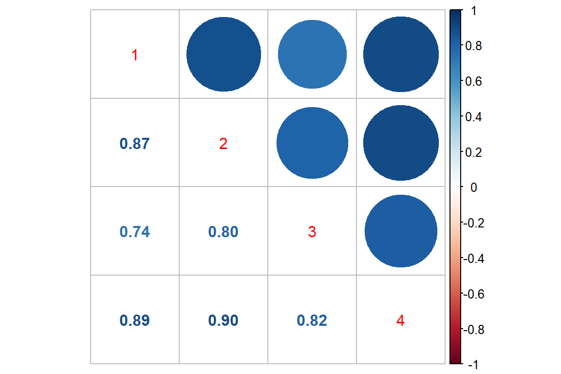
Log Scale
df_long %>%
  dplyr::mutate(rate_wk = log(seizure.rate + 1)) %>%
  dplyr::select(subject, period, rate_wk) %>%
  tidyr::spread(key = period,
                value = rate_wk) %>%
  dplyr::select(-subject) %>%
  cor() %>%
  corrplot::corrplot.mixed()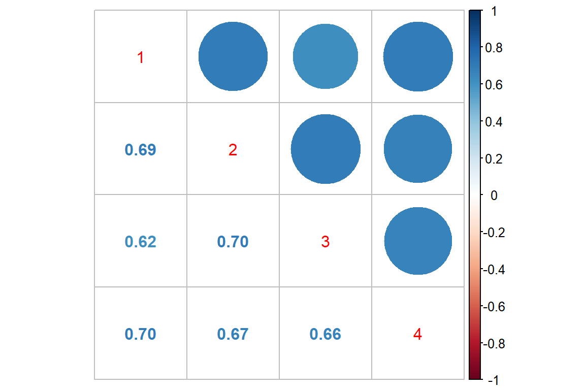
17.2.2 Visualize
17.2.2.1 Outcome on the Raw Scale
There appear to be quite a few extreme values or outliers, particularly for the Progabide group during period one.
Since the outcome is truely a COUNT, we will model it with a Poisson distribution combined with a LOG link.
df_long %>%
  ggplot(aes(x = period,
             y = seizure.rate)) +
  geom_boxplot() +
  theme_bw() +
  facet_grid(.~ treatment)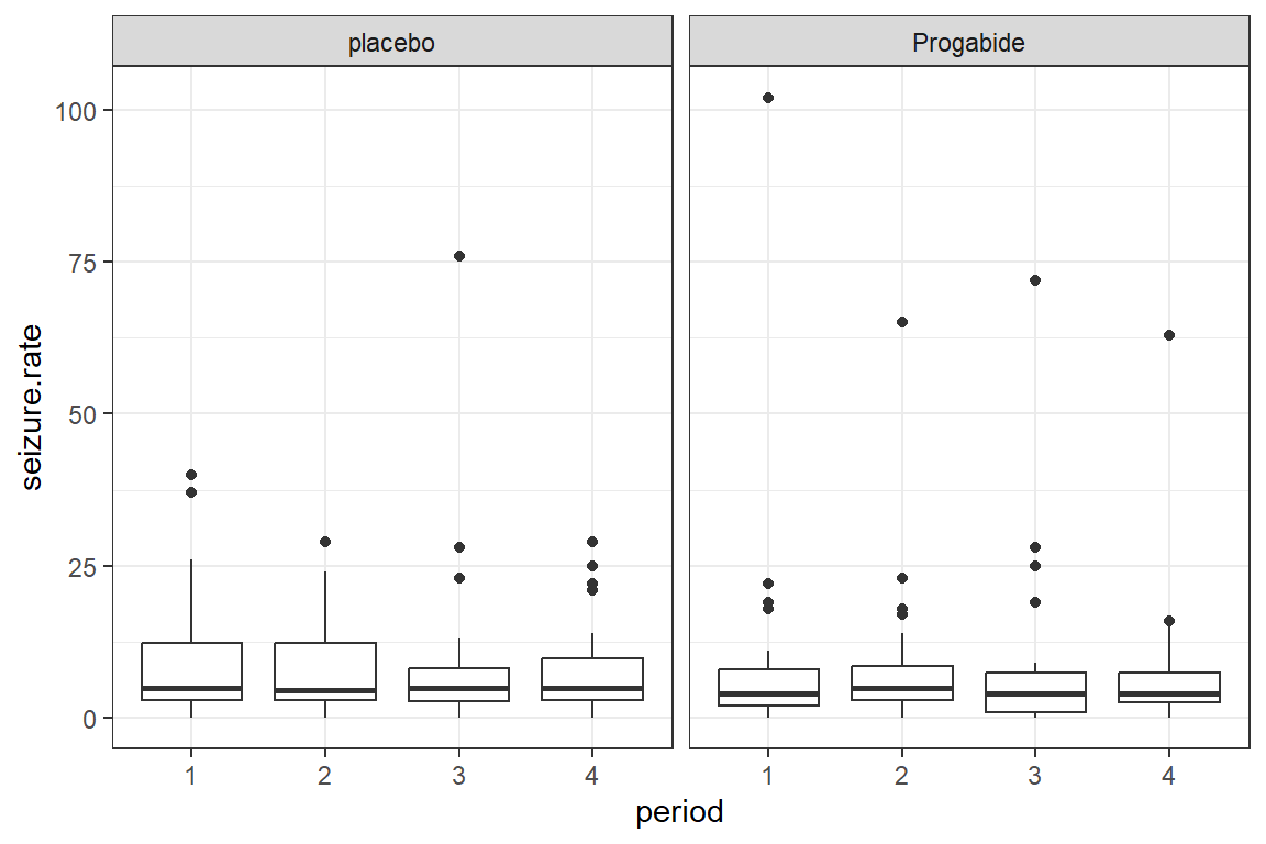
To investigate possible outliers, we should transform the outcome with the log function first.
Note: Since some participants reported no seizures during a two week period and the
log(0)is unndefinded, we must add some amount to the values before transforming. Here we have chosen to add the value of \(1\).
df_long %>%
  ggplot(aes(x = period,
             y = log(seizure.rate + 1))) +
  geom_boxplot() +

  theme_bw() +
  facet_grid(.~ treatment)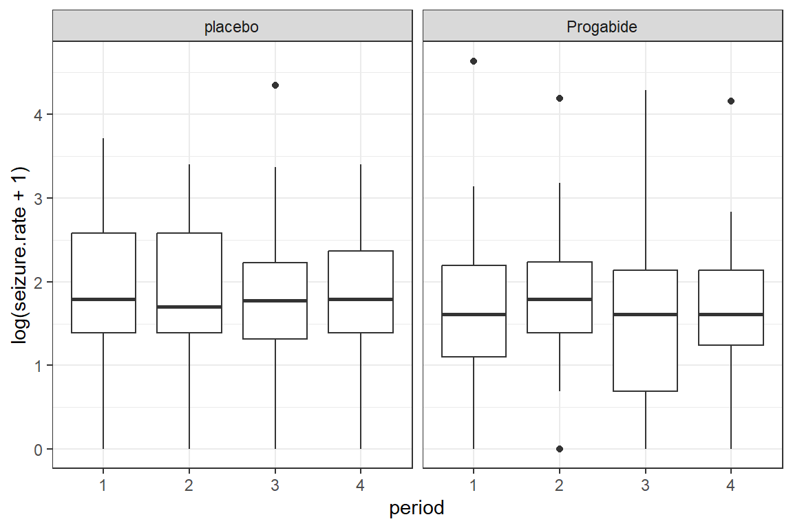
df_long %>%
  ggplot(aes(x = period,
             y = log(seizure.rate + 1))) +
  geom_line(aes(group = subject)) +
  theme_bw() +
  facet_grid(.~ treatment)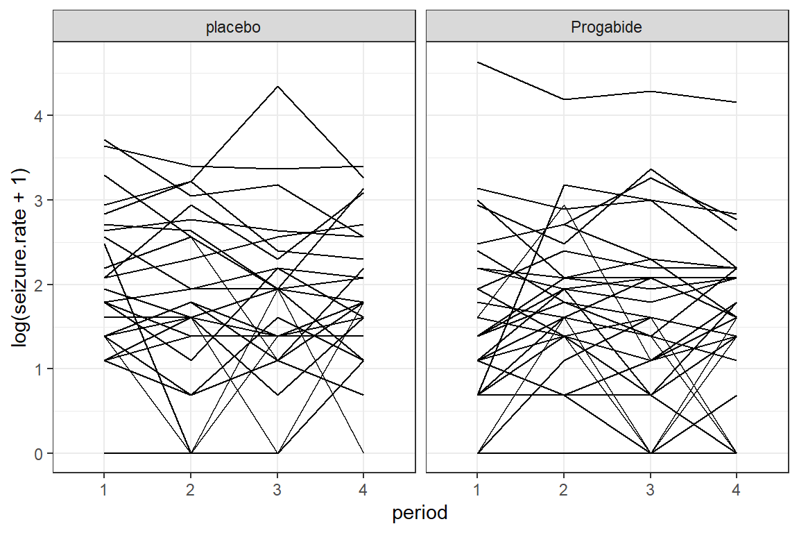
df_long %>%
  ggplot(aes(x = period,
             y = log(seizure.rate + 1))) +
  geom_smooth(aes(group = subject),
              method = "lm",
              se = FALSE) +
  geom_smooth(aes(group = 1),
              color = "red",
              size = 1.5,
              method = "lm",
              se = FALSE) +
  theme_bw() +
  facet_grid(.~ treatment)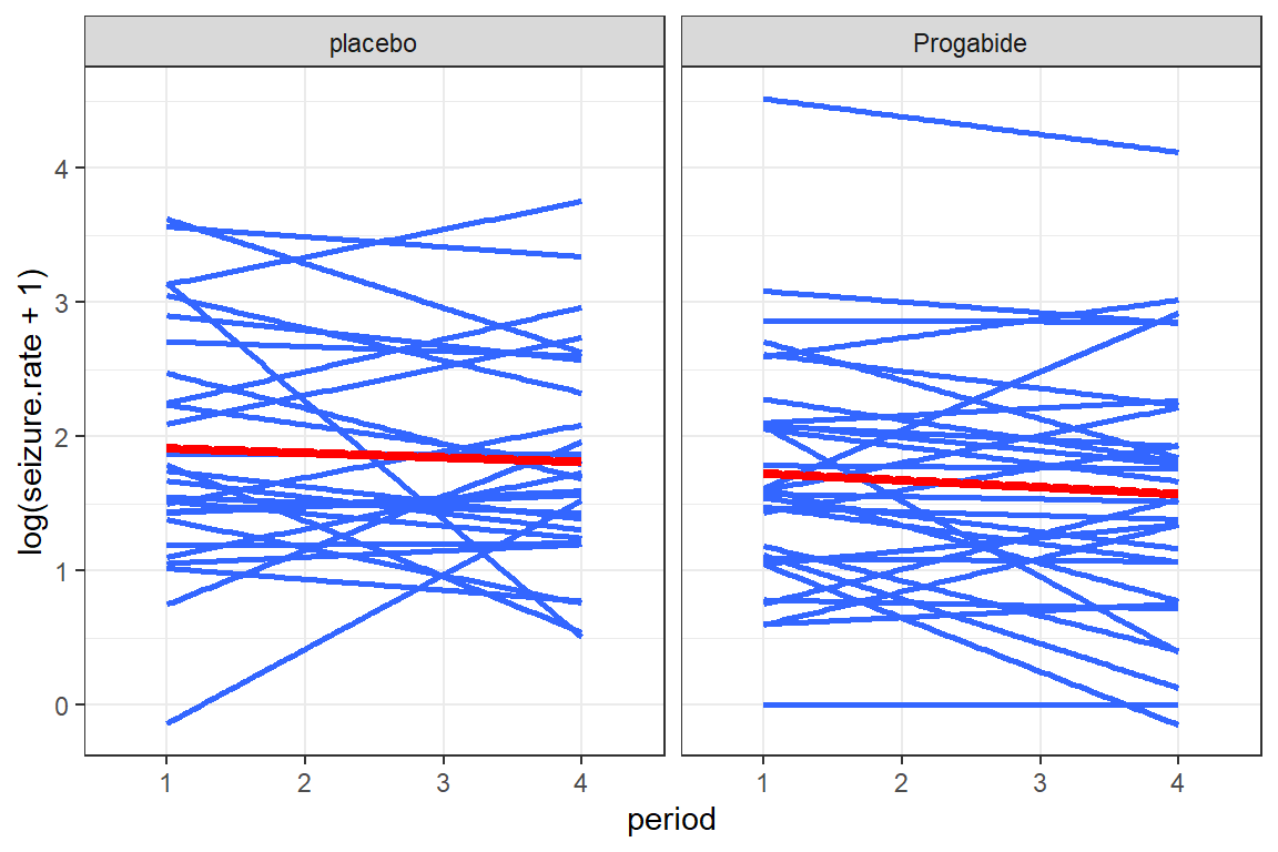
17.3 Poisson Regression (GLM)
Note: THIS IS NEVER APPROPRIATE TO CONDUCT A GLM ON REPEATED MEASURES. THIS IS DONE FOR ILLUSTRATION PURPOSES ONLY!
17.3.1 Fit the model
fit_glm <- glm(seizure.rate ~ base + age + treatment + offset(per),
               data = df_long,
               family = poisson(link = "log"))

summary(fit_glm)
Call:
glm(formula = seizure.rate ~ base + age + treatment + offset(per),
    family = poisson(link = "log"), data = df_long)

Coefficients:
                    Estimate Std. Error z value Pr(>|z|)
(Intercept)        -0.130616   0.135619   -0.96   0.3355
base                0.022652   0.000509   44.48  < 2e-16 ***
age                 0.022740   0.004024    5.65  1.6e-08 ***
treatmentProgabide -0.152701   0.047805   -3.19   0.0014 **
---
Signif. codes:  0 '***' 0.001 '**' 0.01 '*' 0.05 '.' 0.1 ' ' 1

(Dispersion parameter for poisson family taken to be 1)

    Null deviance: 2521.75  on 235  degrees of freedom
Residual deviance:  958.46  on 232  degrees of freedom
AIC: 1732

Number of Fisher Scoring iterations: 5
17.3.2 Tabulate the Model Parameters
Incident Rate Ratio | Log Scale | ||||||||
|---|---|---|---|---|---|---|---|---|---|
Variable | IRR | 95% CI | b | (SE) | Wald | LRT | VIF | ||
(Intercept) | 0.88 | [0.67, 1.14] | -0.13 | (0.14) | .335 | ||||
base | 1.02 | [1.02, 1.02] | 0.02 | (0.00) | < .001*** | < .001*** | 1.17 | ||
age | 1.02 | [1.01, 1.03] | 0.02 | (0.00) | < .001*** | < .001*** | 1.25 | ||
treatment | .001** | 1.11 | |||||||
placebo | — | — | — | — | |||||
Progabide | 0.86 | [0.78, 0.94] | < .001 | (0.05) | .001** | ||||
pseudo-R² | .999 | ||||||||
Note. N = 236. CI = confidence interval; VIF = variance inflation factor. Significance denotes Wald t-tests for individual parameter estimates, as well as Likelihood Ratio Tests (LRT) for single-predictor deletion. Coefficient of determination displays Nagelkerke's pseudo-R². | |||||||||
* p < .05. ** p < .01. *** p < .001. | |||||||||
17.4 Generalized Estimating Equations (GEE)
17.4.1 Match Poisson Regresssion (GLM)
- correlation structure:
independence - scale parameter = \(1\)
fit_gee_ind_s1 <- geepack::geeglm(seizure.rate ~ base + age + treatment + offset(per),
                                  data = df_long,
                                  family = poisson(link = "log"),
                                  id = subject,
                                  waves = period,
                                  corstr = "independence",
                                  scale.fix = TRUE)

summary(fit_gee_ind_s1)
Call:
geepack::geeglm(formula = seizure.rate ~ base + age + treatment +
    offset(per), family = poisson(link = "log"), data = df_long,
    id = subject, waves = period, corstr = "independence", scale.fix = TRUE)

 Coefficients:
                   Estimate  Std.err   Wald Pr(>|W|)
(Intercept)        -0.13062  0.36515   0.13     0.72
base                0.02265  0.00124 336.05   <2e-16 ***
age                 0.02274  0.01158   3.86     0.05 *
treatmentProgabide -0.15270  0.17111   0.80     0.37
---
Signif. codes:  0 '***' 0.001 '**' 0.01 '*' 0.05 '.' 0.1 ' ' 1

Correlation structure = independence
Scale is fixed.

Number of clusters:   59  Maximum cluster size: 4
17.4.2 Change Correlation Sturucture
- correlation structure:
exchangeable - scale parameter = \(1\)
fit_gee_exc_s1 <- geepack::geeglm(seizure.rate ~ base + age + treatment + offset(per),
                           data = df_long,
                           family = poisson(link = "log"),
                           id = subject,
                                  waves = period,
                           corstr = "exchangeable",
                           scale.fix = TRUE)

summary(fit_gee_exc_s1)
Call:
geepack::geeglm(formula = seizure.rate ~ base + age + treatment +
    offset(per), family = poisson(link = "log"), data = df_long,
    id = subject, waves = period, corstr = "exchangeable", scale.fix = TRUE)

 Coefficients:
                   Estimate  Std.err   Wald Pr(>|W|)
(Intercept)        -0.13062  0.36515   0.13     0.72
base                0.02265  0.00124 336.05   <2e-16 ***
age                 0.02274  0.01158   3.86     0.05 *
treatmentProgabide -0.15270  0.17111   0.80     0.37
---
Signif. codes:  0 '***' 0.001 '**' 0.01 '*' 0.05 '.' 0.1 ' ' 1

Correlation structure = exchangeable
Scale is fixed.

  Link = identity

Estimated Correlation Parameters:
      Estimate Std.err
alpha    0.141  0.0415
Number of clusters:   59  Maximum cluster size: 4
17.4.2.1 Interpretation
“For this example, the estimates of standard errors under the independence are about half of the corresponding robust estimates, and the the situation improves only a little when an exchangeable structure is fitted. Using naive standard errors leads, in particular, to a highly significant treatment effect which disappears when the robust estimates are used.”
17.4.3 Estimate the Additional Scale Parameter
“The problem with the GEE approach here, using either the independence or exchangeable correlation structure lies in constraining the scale parameter to be one. For these data there is overdispersion (variance is larger than the mean value) which has to be accommodated by allowing this parameter to be freely estimated.”
- correlation structure:
exchangeable - scale parameter = freely estimated
fit_gee_exc_sf <- geepack::geeglm(seizure.rate ~ base + age + treatment + offset(per),
                           data = df_long,
                           family = poisson(link = "log"),
                           id = subject,
                                  waves = period,
                           corstr = "exchangeable",
                           scale.fix = FALSE)

summary(fit_gee_exc_sf)
Call:
geepack::geeglm(formula = seizure.rate ~ base + age + treatment +
    offset(per), family = poisson(link = "log"), data = df_long,
    id = subject, waves = period, corstr = "exchangeable", scale.fix = FALSE)

 Coefficients:
                   Estimate  Std.err   Wald Pr(>|W|)
(Intercept)        -0.13062  0.36515   0.13     0.72
base                0.02265  0.00124 336.05   <2e-16 ***
age                 0.02274  0.01158   3.86     0.05 *
treatmentProgabide -0.15270  0.17111   0.80     0.37
---
Signif. codes:  0 '***' 0.001 '**' 0.01 '*' 0.05 '.' 0.1 ' ' 1

Correlation structure = exchangeable
Estimated Scale Parameters:

            Estimate Std.err
(Intercept)        5    1.55
  Link = identity

Estimated Correlation Parameters:
      Estimate Std.err
alpha    0.397   0.067
Number of clusters:   59  Maximum cluster size: 4
“When this is done (scale parameter is freely estimated) it gives the last set of results shown above. The estimate of \(\phi\) is 5.”
17.4.4 Compare Models
apaSupp::tab_gees(list("Independence" = fit_gee_ind_s1,
                       "Exchg, fixed" = fit_gee_exc_s1,
                       "Exchg, freed" = fit_gee_exc_sf),
                  narrow = TRUE,
                  caption = "Estimates on Odds-Ratio Scale")
| Independence | Exchg, fixed | Exchg, freed | |||
|---|---|---|---|---|---|---|
IRR | 95% CI | IRR | 95% CI | IRR | 95% CI | |
(Intercept) | 0.88 | [0.43, 1.80] | 0.88 | [0.43, 1.80] | 0.88 | [0.43, 1.80] |
base | 1.02 | [1.02, 1.03]*** | 1.02 | [1.02, 1.03]*** | 1.02 | [1.02, 1.03]*** |
age | 1.02 | [1.00, 1.05]* | 1.02 | [1.00, 1.05]* | 1.02 | [1.00, 1.05]* |
treatment | ||||||
placebo | — | — | — | — | — | — |
Progabide | 0.86 | [0.61, 1.20] | 0.86 | [0.61, 1.20] | 0.86 | [0.61, 1.20] |
Note. | ||||||
* p < .05. ** p < .01. *** p < .001. | ||||||