5 MLM, 2-levels: Pupil Popularity

Download/install a new GitHub package

install.packages("devtools")
devtools::install_github("sarbearschwartz/apaSupp") # updated 9/17/2025

Load/activate these packages

library(haven)  
library(tidyverse)    
library(flextable)
library(apaSupp)      # Not on CRAN, on GitHub (see above)
library(performance)
library(lme4)        
library(lmerTest)   
library(insight)
library(interactions)
library(effects)
library(sjPlot)

5.1 Background

The text “Multilevel Analysis: Techniques and Applications, Third Edition” (Hox, Moerbeek, and Van de Schoot 2017) has a companion website which includes links to all the data files used throughout the book (housed on the book’s GitHub repository).

The following example is used through out (Hox, Moerbeek, and Van de Schoot 2017)’s chapater 2.

From Appendix E:

The popularity data in popular2.sav are simulated data for 2000 pupils (pupil) in 100 schools (class). The purpose is to offer a very simple example for multilevel regression analysis.

The main OUTCOME or DEPENDENT VARIABLE (DV) is the pupil popularity, a popularity rating on a scale of 1-10 derived by a sociometric procedure. Typically, a sociometric procedure asks all pupils in a class to rate all the other pupils, and then assigns the average received popularity rating to each pupil (pupular). Because of the sociometric procedure, group effects as apparent from higher level variance components are rather strong. There is a second outcome variable, pupil popularity as rated by their teacher (popteach), on a scale from 1-10.

The PREDICTORS or INDEPENDENT VARIABLES (IVs) are:

pupil gender (sex) only two levels: boy = 0, girl = 1

pupil extroversion (extrav) 10-point scale (whole number) as rated by the teacher, higher values correspond to more extroverted

teacher experience (texp) in years, reported as a whole number

The popularity data have been generated to be a ‘nice’ well-behaved data set: the sample sizes at both levels are sufficient, the residuals have a normal distribution, and the multilevel effects are strong.

Note: We will ignore the centered and standardized variables, which start with a capital Z or C.

data_raw <- haven::read_sav("data/popular2.sav") %>% 
  haven::as_factor() %>%             # retain the labels from SPSS --> factor
  haven::zap_label()                 # drop the varaible labels from SPSS

tibble::glimpse(data_raw)

Rows: 2,000
Columns: 15
$ pupil     <dbl> 1, 2, 3, 4, 5, 6, 7, 8, 9, 10, 11, 12, 13, 14, 15, 16, 17, 1…
$ class     <dbl> 1, 1, 1, 1, 1, 1, 1, 1, 1, 1, 1, 1, 1, 1, 1, 1, 1, 1, 1, 1, …
$ extrav    <dbl> 5, 7, 4, 3, 5, 4, 5, 4, 5, 5, 5, 5, 5, 5, 5, 6, 4, 4, 7, 4, …
$ sex       <fct> girl, boy, girl, girl, girl, boy, boy, boy, boy, boy, girl, …
$ texp      <dbl> 24, 24, 24, 24, 24, 24, 24, 24, 24, 24, 24, 24, 24, 24, 24, …
$ popular   <dbl> 6.3, 4.9, 5.3, 4.7, 6.0, 4.7, 5.9, 4.2, 5.2, 3.9, 5.7, 4.8, …
$ popteach  <dbl> 6, 5, 6, 5, 6, 5, 5, 5, 5, 3, 5, 5, 5, 6, 5, 5, 2, 3, 7, 4, …
$ Zextrav   <dbl> -0.1703149, 1.4140098, -0.9624772, -1.7546396, -0.1703149, -…
$ Zsex      <dbl> 0.9888125, -1.0108084, 0.9888125, 0.9888125, 0.9888125, -1.0…
$ Ztexp     <dbl> 1.48615283, 1.48615283, 1.48615283, 1.48615283, 1.48615283, …
$ Zpopular  <dbl> 0.88501327, -0.12762911, 0.16169729, -0.27229230, 0.66801848…
$ Zpopteach <dbl> 0.66905609, -0.04308451, 0.66905609, -0.04308451, 0.66905609…
$ Cextrav   <dbl> -0.215, 1.785, -1.215, -2.215, -0.215, -1.215, -0.215, -1.21…
$ Ctexp     <dbl> 9.737, 9.737, 9.737, 9.737, 9.737, 9.737, 9.737, 9.737, 9.73…
$ Csex      <dbl> 0.5, -0.5, 0.5, 0.5, 0.5, -0.5, -0.5, -0.5, -0.5, -0.5, 0.5,…

5.1.1 Unique Identifiers

We will restrict ourselves to a few of the variables and create a unique identifier variable for each student.

data_pop <- data_raw %>%   
  dplyr::mutate(id = paste(class, pupil,
                           sep = "_") %>%   # create a unique id for each student (char)
                  factor()) %>%             # declare id is a factor
  dplyr::select(id, pupil:popteach)         # reduce the variables included

tibble::glimpse(data_pop)

Rows: 2,000
Columns: 8
$ id       <fct> 1_1, 1_2, 1_3, 1_4, 1_5, 1_6, 1_7, 1_8, 1_9, 1_10, 1_11, 1_12…
$ pupil    <dbl> 1, 2, 3, 4, 5, 6, 7, 8, 9, 10, 11, 12, 13, 14, 15, 16, 17, 18…
$ class    <dbl> 1, 1, 1, 1, 1, 1, 1, 1, 1, 1, 1, 1, 1, 1, 1, 1, 1, 1, 1, 1, 2…
$ extrav   <dbl> 5, 7, 4, 3, 5, 4, 5, 4, 5, 5, 5, 5, 5, 5, 5, 6, 4, 4, 7, 4, 8…
$ sex      <fct> girl, boy, girl, girl, girl, boy, boy, boy, boy, boy, girl, g…
$ texp     <dbl> 24, 24, 24, 24, 24, 24, 24, 24, 24, 24, 24, 24, 24, 24, 24, 2…
$ popular  <dbl> 6.3, 4.9, 5.3, 4.7, 6.0, 4.7, 5.9, 4.2, 5.2, 3.9, 5.7, 4.8, 5…
$ popteach <dbl> 6, 5, 6, 5, 6, 5, 5, 5, 5, 3, 5, 5, 5, 6, 5, 5, 2, 3, 7, 4, 6…

5.1.2 Structure and variables

Its a good idea to visually inspect the first few lines in the datast to get a sense of how it is organized.

data_pop %>%  
  psych::headTail(top = 25, bottom = 5) %>% 
  flextable::flextable() %>% 
  apaSupp::theme_apa(caption = "Partial Data Printout")

**Table 5.1**
Partial Data Printout
id	pupil	class	extrav	sex	texp	popular	popteach
1_1	1	1	5	girl	24	6.3	6
1_2	2	1	7	boy	24	4.9	5
1_3	3	1	4	girl	24	5.3	6
1_4	4	1	3	girl	24	4.7	5
1_5	5	1	5	girl	24	6	6
1_6	6	1	4	boy	24	4.7	5
1_7	7	1	5	boy	24	5.9	5
1_8	8	1	4	boy	24	4.2	5
1_9	9	1	5	boy	24	5.2	5
1_10	10	1	5	boy	24	3.9	3
1_11	11	1	5	girl	24	5.7	5
1_12	12	1	5	girl	24	4.8	5
1_13	13	1	5	boy	24	5	5
1_14	14	1	5	girl	24	5.5	6
1_15	15	1	5	girl	24	6	5
1_16	16	1	6	girl	24	5.7	5
1_17	17	1	4	boy	24	3.2	2
1_18	18	1	4	boy	24	3.1	3
1_19	19	1	7	girl	24	6.6	7
1_20	20	1	4	boy	24	4.8	4
2_1	1	2	8	girl	14	6.4	6
2_2	2	2	4	boy	14	2.4	3
2_3	3	2	6	boy	14	3.7	4
2_4	4	2	5	girl	14	4.4	4
2_5	5	2	5	girl	14	4.3	4
	...	...	...		...	...	...
100_16	16	100	4	girl	7	4.3	5
100_17	17	100	4	boy	7	2.6	2
100_18	18	100	8	girl	7	6.7	7
100_19	19	100	5	boy	7	2.9	3
100_20	20	100	9	boy	7	5.3	5

Visual inspection reveals that most of the variables are measurements at level 1 and apply to specific pupils (extrav, sex, popular, and popteach), while the teacher’s years of experience is a level 2 variable since it applies to the entire class. Notice how the texp variable is identical for all pupils in the same class. This is call Disaggregated data.

5.2 Exploratory Data Analysis

5.2.1 Summarize Descriptive Statistics

5.2.1.1 The `apaSupp` package

Most posters, journal articles, and reports start with a table of descriptive statistics. Since it tends to come first, this type of table is often refered to as Table 1.

**Table 5.2**
Descriptive statistics, aggregate over entire sample
	NA	M	SD	min	Q1	Mdn	Q3	max
Teacher's Experience	0	14.26	6.55	2.00	8.00	15.00	20.00	25.00
Pupil's Extroversion	0	5.21	1.26	1.00	4.00	5.00	6.00	10.00
Pupil's Popularity	0	5.08	1.38	0.00	4.10	5.10	6.00	9.50
Note. N = 2000. NA = not available or missing; Mdn = median; Q1 = 25th percentile; Q3 = 75th percentile.

data_pop %>% 
  dplyr::select(sex,
                "Teacher Experience" = texp, 
                "Pupil Extroversion" = extrav, 
                "Pupil Popularity"   = popular) %>% 
  apaSupp::tab1(split = "sex",
                total_last = FALSE,
                caption    = "Compare genders on four main variables")

5.2.2 Visualizations of Raw Data

5.2.2.1 Ignore Clustering

5.2.2.1.1 Scatterplots

For a first look, its useful to plot all the data points on a single scatterplot as displayed in Figure 5.1. Due to ganularity in the rating scale, many points end up being plotted on top of each other (overplotted), so its a good idea to use geom_count() rather than geom_point() so the size of the dot can convey the number of points at that location (Wickham et al. 2025).

# Disaggregate: pupil (level 1) only, ignore level 2's existance
# extroversion treated: continuous measure
data_pop %>% 
  ggplot() +
  aes(x = extrav,                                # x-axis variable
      y = popular) +                             # y-axis variable
  geom_count() +                                 # POINTS w/ SIZE = COUNT
  geom_smooth(method = "lm") +                   # linear regression line
  theme_bw() +                                   # white background  
  labs(x    = "extroversion (10 pt scale)",      # x-axis label
       y    = "Popularity, Sociometric Score",   # y-axis label
       size = "Count") +                         # legend key's title  
  theme(legend.position = c(0.9, 0.2),                          # key at
        legend.background = element_rect(color = "black")) +    # key box 
  scale_x_continuous(breaks = seq(from = 0, to = 10, by = 1)) + # x-ticks
  scale_y_continuous(breaks = seq(from = 0, to = 10, by = 2))   # y-ticks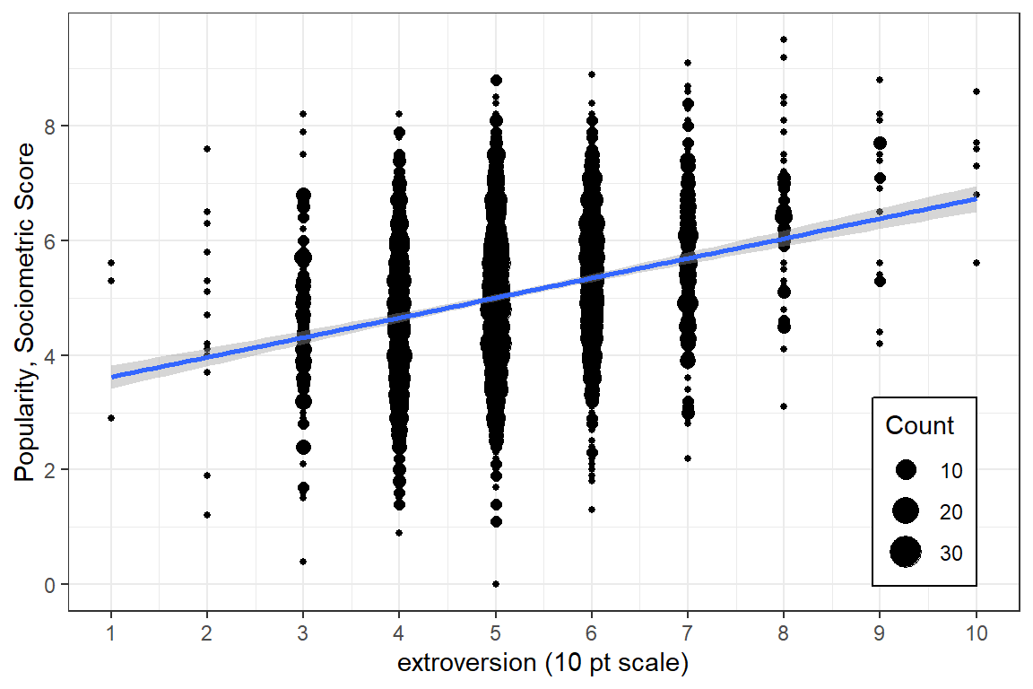

Figure 5.1
Disaggregate: pupil level only with extroversion treated as an continuous measure.

5.2.2.1.2 Density Plots

When the degree of overplotting as high as it is in Figure 5.1, it can be useful to represent the data with density contours as seen in Figure 5.2. I’ve chosen to leave the points displayed in this redition, but color them much lighter so that they are present, but do not detract from the pattern of association.

data_pop %>% 
  ggplot() +
  aes(x = extrav,                                # x-axis variable
      y = popular) +                             # y-axis variable
  geom_count(color = "gray") +                   # POINTS w/ SIZE = COUNT
  geom_density2d() +                             # DENSITY CURVES 
  geom_smooth(method = "lm", color = "red") +    # linear regression line
  theme_bw() +                                   # white background  
  labs(x    = "Extroversion (10 pt scale)",      # x-axis label
       y    = "Popularity, Sociometric Score") + # y-axis label 
  guides(size = FALSE)  +                        # don't include a legend
  scale_x_continuous(breaks = seq(from = 0, to = 10, by = 1)) + # x-ticks
  scale_y_continuous(breaks = seq(from = 0, to = 10, by = 2))   # y-ticks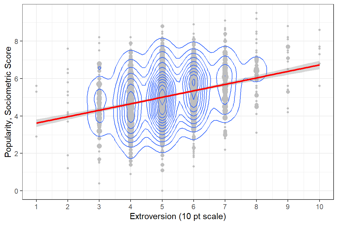

Figure 5.2
Disaggregate: pupil level only with extroversion treated as an continuous measure.

5.2.2.1.3 Histograms, stacked

The argument could be made that the extroversion score should be treated as an ordinal factor instead of as a truly continuous scale since the only valid values are the whole number 1 through 10 and there is no assurance that these category assignments represent a true ratio measurement scale. However, we must keep in mind that this was an observational study, ans as such, the number of pupils assignment each level of extroversion is not equal.

# count the number of pupils in assigned each extroversion value, 1:10
data_pop %>%
  dplyr::group_by(extrav) %>%
  dplyr::summarise(Count = n_distinct(id),
                   Percent  = 100 * Count / 2000) %>%
  flextable::flextable() %>%
  apaSupp::theme_apa(caption = "Distribution of extroversion in pupils")

**Table 5.3**
Distribution of extroversion in pupils
extrav	Count	Percent
1.00	3	0.15
2.00	13	0.65
3.00	119	5.95
4.00	423	21.15
5.00	688	34.40
6.00	478	23.90
7.00	194	9.70
8.00	58	2.90
9.00	18	0.90
10.00	6	0.30

5.2.2.1.4 Boxplots

Figure 5.3 displays the same data as Figure 5.1, but uses boxplots for the distribution of scores at each level of extroversion.

# Disaggregate: pupil (level 1) only, ignore level 2's existance
# extroversion treated: ordinal factor
ggplot(data_pop,                        # dataset's name
       aes(x    = factor(extrav),       # x-axis values - make factor!
           y    = popular,              # y-axis values
           fill = factor(extrav))) +    # makes seperate boxes
  geom_boxplot(varwidth = TRUE) +       # draw boxplots instead of points
  theme_bw() +                          # white background  
  guides(fill = FALSE)  +               # don't include a legend
  scale_y_continuous(breaks = seq(from = 0, to = 10, by = 2)) +  # y-ticks
  labs(x = "extroversion (10 pt scale)",                    # x-axis label
       y = "Popularity, Sociometric Score") +               # y-axis label
  scale_fill_brewer(palette = "Spectral", direction = 1)    # select color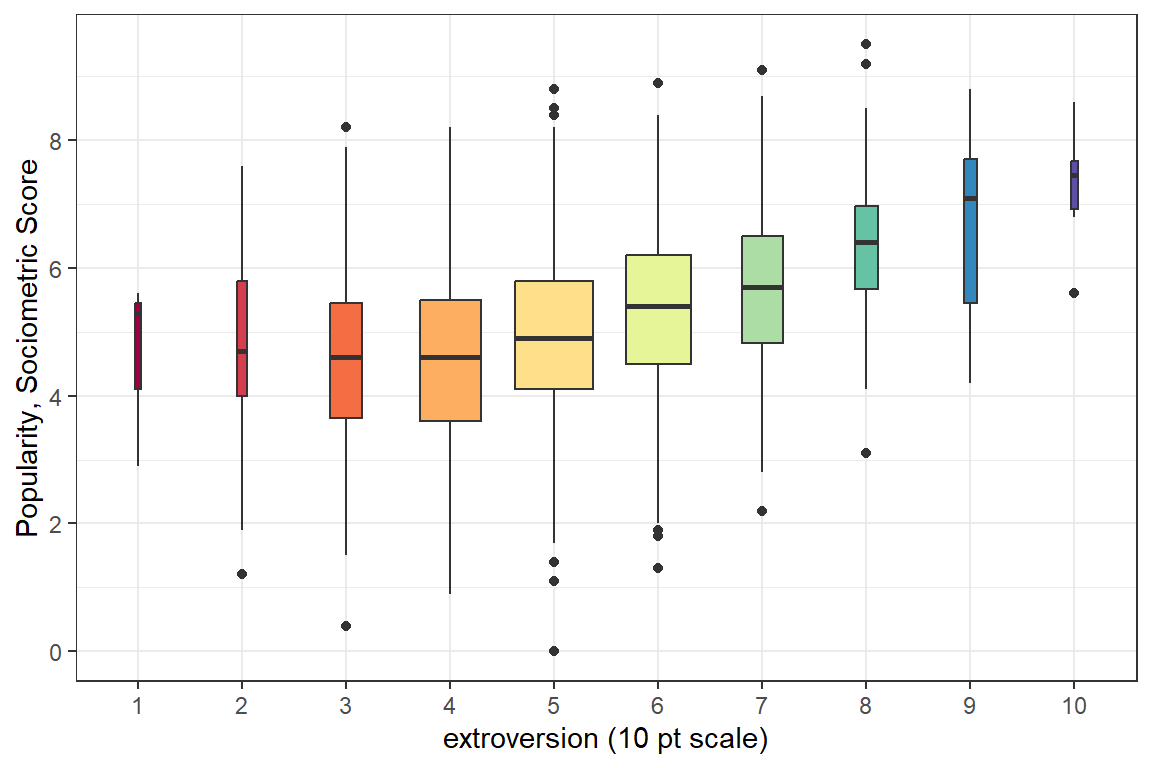

Disaggregate: pupil level only with extroversion treated as an ordinal factor. The width of the boxes are proportional to the square-roots of the number of observations each box represents.

Figure 5.3
Disaggregate: pupil level only with extroversion treated as an ordinal factor. The width of the boxes are proportional to the square-roots of the number of observations each box represents.

5.2.3 Consider Clustering

5.2.3.1 Scatterplots

Up to this point, all investigation of this dataset has been only at the pupil level and any nesting or clustering within classes has been ignored. Plotting is a good was to start to get an idea of the class-to-class variability.

# compare the first 9 classrooms becuase all of there are too many at once
data_pop %>% 
  dplyr::filter(class <= 9) %>%                  # select ONLY NINE classes
  ggplot(aes(x = extrav,                         # x-axis values
             y = popular)) +                     # y-axis values
  geom_count() +                                 # POINTS w/ SIZE = COUNT
  geom_smooth(method = "lm", color = "red") +    # linear regression line
  theme_bw() +                                   # white background  
  labs(x    = "extroversion (10 pt scale)",      # x-axis label
       y    = "Popularity, Sociometric Score",   # y-axis label
       size = "Count") +                         # legend key's title  
  guides(size = FALSE)  +                        # don't include a legend
  scale_x_continuous(breaks = seq(from = 0, to = 10, by = 3)) + # x-ticks
  scale_y_continuous(breaks = seq(from = 0, to = 10, by = 3)) + # y-ticks
  facet_wrap(~ class, 
             labeller = label_both) +
  theme(strip.background = element_rect(colour = NA, 
                                        fill   = NA))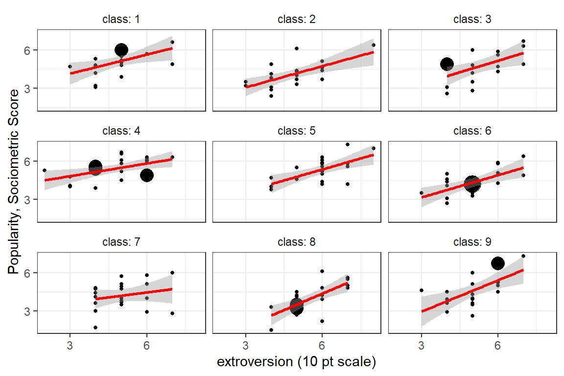

Illustration of the degree of class level variability in the association between extroversion and popularity. Each panel represents a class and each point a pupil in that class. First nice classes shown.

Figure 5.4
Illustration of the degree of class level variability in the association between extroversion and popularity. Each panel represents a class and each point a pupil in that class. First nice classes shown.

# select specific classes by number for illustration purposes
data_pop %>% 
  dplyr::filter(class %in% c(15, 25, 33, 
                             35, 51, 64, 
                             76, 94, 100)) %>% 
  ggplot(aes(x = extrav,                         # x-axis values
             y = popular)) +                     # y-axis values
  geom_count() +                                 # POINTS w/ SIZE = COUNT
  geom_smooth(method = "lm", color = "red") +    # linear regression line
  theme_bw() +                                   # white background  
  labs(x    = "extroversion (10 pt scale)",      # x-axis label
       y    = "Popularity, Sociometric Score",   # y-axis label
       size = "Count") +                         # legend key's title  
  guides(size = FALSE)  +                        # don't include a legend
  scale_x_continuous(breaks = seq(from = 0, to = 10, by = 3)) + # x-ticks
  scale_y_continuous(breaks = seq(from = 0, to = 10, by = 3)) + # y-ticks
  facet_wrap(~ class)  +
  theme(strip.background = element_blank(),
        strip.text       = element_blank())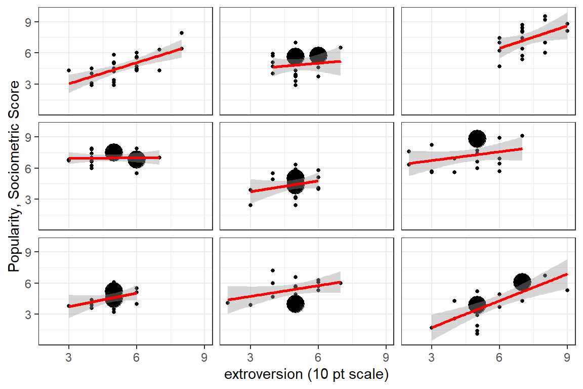

Figure 5.5
Illustration of the degree of class level variability in the association between extroversion and popularity. Each panel represents a class and each point a pupil in that class. A set of nine classes was chosen to show a sampling of variability. The facet labels are not shown as the identification number probably would not be advisable for a general publication.

5.2.3.2 Cluster-wise Regression

# compare all 100 classrooms via linear model for each
data_pop %>% 
  ggplot(aes(x     = extrav,                      # x-axis values
             y     = popular,                     # y-axis values
             group = class)) +                    # GROUPs for LINES
  geom_smooth(method = "lm",                      # linear regression line
              color  = "gray40",
              size   = 0.4,
              se     = FALSE) + 
  theme_bw() +                                   # white background  
  labs(x    = "extroversion (10 pt scale)",      # x-axis label
       y    = "Popularity, Sociometric Score") + # y-axis label
  scale_x_continuous(breaks = seq(from = 0, to = 10, by = 2)) + # x-ticks
  scale_y_continuous(breaks = seq(from = 0, to = 10, by = 2))   # y-ticks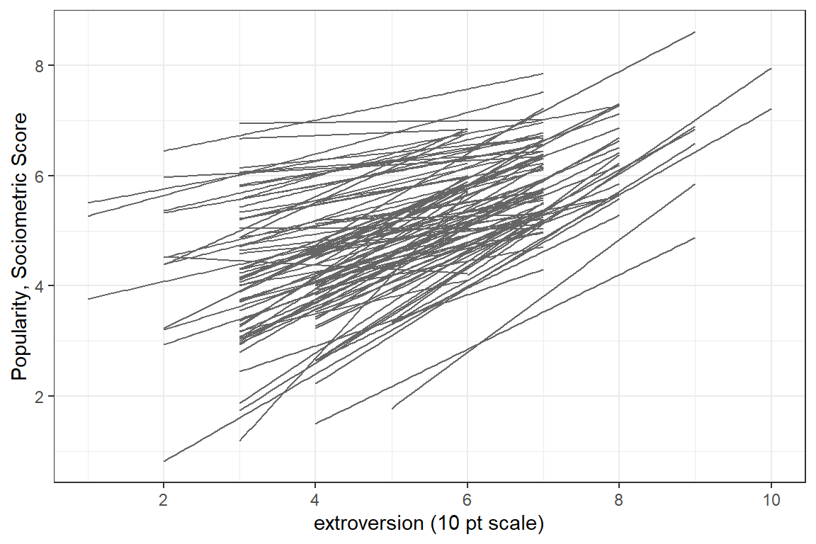

Figure 5.6
Spaghetti plot of seperate, independent linear models for each of the 100 classes.

A helpful resource for choosing colors to use in plots: R color cheatsheet

# compare all 100 classrooms via independent linear models
data_pop %>% 
  dplyr::mutate(texp3 = cut(texp, 
                            breaks = c(0, 10, 18, 30)) %>% 
                  factor(labels = c("< 10 yrs", 
                                    "10 - 18 yrs", 
                                    "> 18 yrs"))) %>% 
  ggplot(aes(x     = extrav,                     # x-axis values
             y     = popular,                    # y-axis values
             group = class)) +                   # GROUPs for LINES
  geom_smooth(aes(color = sex),
              size   = 0.3,
              method = "lm",                     # linear regression line
              se     = FALSE) + 
  theme_bw() +                                   # white background  
  labs(x    = "extroversion (10 pt scale)",      # x-axis label
       y    = "Popularity, Sociometric Score") + # y-axis label
  guides(color = FALSE) +                        # don't include a legend
  scale_x_continuous(breaks = seq(from = 0, to = 10, by = 3)) + # x-ticks
  scale_y_continuous(breaks = seq(from = 0, to = 10, by = 3)) + # y-ticks
  scale_color_manual(values = c("dodgerblue", "maroon1")) +
  facet_grid(texp3 ~ sex)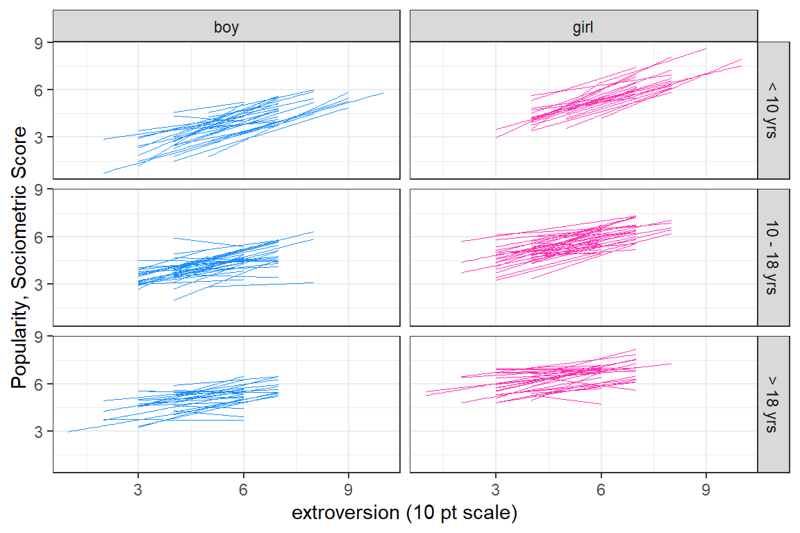

Spaghetti plot of seperate, independent linear models for each of the 100 classes. Seperate panels are used to untangle the 'hairball' in the previous figure. The columns are seperated by the pupils' gender and the rows by the teacher's experince in years.

Figure 5.7
Spaghetti plot of seperate, independent linear models for each of the 100 classes. Seperate panels are used to untangle the ‘hairball’ in the previous figure. The columns are seperated by the pupils’ gender and the rows by the teacher’s experince in years.

5.3 Single-level Regression Analysis

5.3.1 Null Model

In a Null, intercept-only, or Empty model, no predictors are included.

5.3.1.1 Equations

Single-Level Regression Equation - Null Model \[ \overbrace{POP_{ij}}^{Outcome} = \underbrace{\beta_{0}}_{\text{Fixed}\atop\text{intercept}} + \underbrace{e_{ij}}_{\text{Random}\atop\text{residuals}} \]

5.3.1.2 Parameters

Type	Parameter of Interest	Estimates This
Fixed	Intercept	$\beta_{0}$
Random	Residual Variance $var[e_{ij}]$	$\sigma^2_{e}$

5.3.1.3 Fit the Model

pop_lm_0 <- lm(popular ~ 1,        #  The 1 represents the intercept
               data = data_pop) 

summary(pop_lm_0)


Call:
lm(formula = popular ~ 1, data = data_pop)

Residuals:
    Min      1Q  Median      3Q     Max 
-5.0765 -0.9765  0.0235  0.9236  4.4235 

Coefficients:
            Estimate Std. Error t value Pr(>|t|)    
(Intercept)  5.07645    0.03091   164.2   <2e-16 ***
---
Signif. codes:  0 '***' 0.001 '**' 0.01 '*' 0.05 '.' 0.1 ' ' 1

Residual standard error: 1.383 on 1999 degrees of freedom

$\hat{\beta_0}$ = 5.08 is the grand mean

pop_glm_0 <- glm(popular ~ 1,        #  The 1 represents the intercept
                 data = data_pop) 

summary(pop_glm_0)


Call:
glm(formula = popular ~ 1, data = data_pop)

Coefficients:
            Estimate Std. Error t value Pr(>|t|)    
(Intercept)  5.07645    0.03091   164.2   <2e-16 ***
---
Signif. codes:  0 '***' 0.001 '**' 0.01 '*' 0.05 '.' 0.1 ' ' 1

(Dispersion parameter for gaussian family taken to be 1.911366)

    Null deviance: 3820.8  on 1999  degrees of freedom
Residual deviance: 3820.8  on 1999  degrees of freedom
AIC: 6974.4

Number of Fisher Scoring iterations: 2

5.3.1.4 Model Fit

performance::performance(pop_lm_0)

# Indices of model performance

AIC    |   AICc |    BIC | R2 | R2 (adj.) |  RMSE | Sigma
---------------------------------------------------------
6974.4 | 6974.4 | 6985.6 |  0 |         0 | 1.382 | 1.383

performance::performance(pop_glm_0)

# Indices of model performance

AIC    |   AICc |    BIC | R2 |  RMSE | Sigma
---------------------------------------------
6974.4 | 6974.4 | 6985.6 |  0 | 1.382 | 1.383

performance::compare_performance(pop_lm_0, pop_glm_0)

# Comparison of Model Performance Indices

Name      | Model |  AIC (weights) | AICc (weights) |  BIC (weights) | R2
-------------------------------------------------------------------------
pop_lm_0  |    lm | 6974.4 (0.500) | 6974.4 (0.500) | 6985.6 (0.500) |  0
pop_glm_0 |   glm | 6974.4 (0.500) | 6974.4 (0.500) | 6985.6 (0.500) |  0

Name      |  RMSE | Sigma | R2 (adj.)
-------------------------------------
pop_lm_0  | 1.382 | 1.383 |         0
pop_glm_0 | 1.382 | 1.383 |

Residual variance:

sigma(pop_lm_0)    # standard deviation of the residuals

[1] 1.382522

sigma(pop_lm_0)^2  # variance of the residuals

[1] 1.911366

$\hat{\sigma_e^2}$ = 1.9114 is residual variance (RMSE is sigma = 1.3825)

Variance Explained:

summary(pop_lm_0)$r.squared

[1] 0

$R^2$ = 0 is the proportion of variance in popularity that is explained by the grand mean alone.

Deviance:

-2 * logLik(pop_lm_0)

'log Lik.' 6970.39 (df=2)

5.3.1.5 Interpretation

The grand average popularity of all pupils in all the classes is 5.08, and there is strong evidence that it is statistically significantly different than zero, $p<.0001$. The mean alone accounts for none of the variance in popularity. The residual variance is the same as the total variance in popularity, 1.9114.

Just to make sure…

mean(data_pop$popular)

[1] 5.07645

var(data_pop$popular)

[1] 1.911366

5.3.2 Add Predictors to the Model

5.3.2.1 Equations

LEVEL 1: Student-specific predictors:

$X_1 = GEN$, pupils’s gender (girl vs. boy)

$X_2 = EXT$, pupil’s extroversion (scale: 1-10)

Single-Level Regression Equation \[ \overbrace{POP_{ij}}^{Outcome} = \underbrace{\beta_{0}}_{\text{Fixed}\atop\text{intercept}} + \underbrace{\beta_{1}}_{\text{Fixed}\atop\text{slope}} \overbrace{GEN_{ij}}^{\text{Predictor 1}} + \underbrace{\beta_{2}}_{\text{Fixed}\atop\text{slope}} \overbrace{EXT_{ij}}^{\text{Predictor 2}} + \underbrace{e_{ij}}_{\text{Random}\atop\text{residuals}} \tag{Hox 2.1} \]

5.3.2.2 Parameters

Type	Parameter of Interest	Estimates This
Fixed	Intercept	$\beta_{0}$
Fixed	Slope or effect of `sex`	$\beta_{1}$
Fixed	Slope or effect of `extrav`	$\beta_{2}$
Random	Residual Variance $var[e_{ij}]$	$\sigma^2_{e}$

5.3.2.3 Fit the Model

pop_lm_1 <- lm(popular ~ sex + extrav,    # implies: 1 + sex + extrav
               data = data_pop) 

summary(pop_lm_1)


Call:
lm(formula = popular ~ sex + extrav, data = data_pop)

Residuals:
    Min      1Q  Median      3Q     Max 
-4.2527 -0.6652 -0.0454  0.7422  3.0473 

Coefficients:
            Estimate Std. Error t value Pr(>|t|)    
(Intercept)  2.78954    0.10355   26.94   <2e-16 ***
sexgirl      1.50508    0.04836   31.12   <2e-16 ***
extrav       0.29263    0.01916   15.28   <2e-16 ***
---
Signif. codes:  0 '***' 0.001 '**' 0.01 '*' 0.05 '.' 0.1 ' ' 1

Residual standard error: 1.077 on 1997 degrees of freedom
Multiple R-squared:  0.3938,    Adjusted R-squared:  0.3932 
F-statistic: 648.6 on 2 and 1997 DF,  p-value: < 2.2e-16

pop_glm_1 <- glm(popular ~ sex + extrav,    # implies: 1 + sex + extrav
                 data = data_pop) 

summary(pop_glm_1)


Call:
glm(formula = popular ~ sex + extrav, data = data_pop)

Coefficients:
            Estimate Std. Error t value Pr(>|t|)    
(Intercept)  2.78954    0.10355   26.94   <2e-16 ***
sexgirl      1.50508    0.04836   31.12   <2e-16 ***
extrav       0.29263    0.01916   15.28   <2e-16 ***
---
Signif. codes:  0 '***' 0.001 '**' 0.01 '*' 0.05 '.' 0.1 ' ' 1

(Dispersion parameter for gaussian family taken to be 1.159898)

    Null deviance: 3820.8  on 1999  degrees of freedom
Residual deviance: 2316.3  on 1997  degrees of freedom
AIC: 5977.4

Number of Fisher Scoring iterations: 2

$\hat{\beta_0}$ = 2.79 is the extrapolated mean for boys with an extroversion score of 0.
$\hat{\beta_1}$ = 1.51 is the mean difference between girls and boys with the same extroversion score.

$\hat{\beta_2}$ = 0.29 is the mean difference for pupils of the same gender that differ in extroversion by one point.

5.3.2.4 Model Fit

Residual variance:

sigma(pop_lm_1)    # standard deviation of the residuals

[1] 1.076985

sigma(pop_lm_1)^2  # variance of the residuals

[1] 1.159898

$\hat{\sigma_e^2}$ = 1.1599 is residual variance (RMSE is sigma)

Variance Explained:

summary(pop_lm_1)$r.squared

[1] 0.393765

Deviance:

-2 * logLik(pop_lm_1)

'log Lik.' 5969.415 (df=4)

$R^2$ = 0.394 is the proportion of variance in popularity that is explained by tha pupils gender and extroversion score.

performance::performance(pop_lm_1)

# Indices of model performance

AIC    |   AICc |    BIC |    R2 | R2 (adj.) |  RMSE | Sigma
------------------------------------------------------------
5977.4 | 5977.4 | 5999.8 | 0.394 |     0.393 | 1.076 | 1.077

Note”: BF = the Bayes factor

performance::compare_performance(pop_lm_0, 
                                 pop_lm_1, 
                                 rank = TRUE)

# Comparison of Model Performance Indices

Name     | Model |    R2 | R2 (adj.) |  RMSE | Sigma | AIC weights
------------------------------------------------------------------
pop_lm_1 |    lm | 0.394 |     0.393 | 1.076 | 1.077 |        1.00
pop_lm_0 |    lm | 0.000 |     0.000 | 1.382 | 1.383 |   3.23e-217

Name     | AICc weights | BIC weights | Performance-Score
---------------------------------------------------------
pop_lm_1 |         1.00 |        1.00 |           100.00%
pop_lm_0 |    3.26e-217 |   8.75e-215 |             0.00%

performance::compare_performance(pop_glm_0, 
                                 pop_glm_1, 
                                 rank = TRUE)

# Comparison of Model Performance Indices

Name      | Model |    R2 |  RMSE | Sigma | AIC weights | AICc weights
----------------------------------------------------------------------
pop_glm_1 |   glm | 0.394 | 1.076 | 1.077 |        1.00 |         1.00
pop_glm_0 |   glm | 0.000 | 1.382 | 1.383 |   3.23e-217 |    3.26e-217

Name      | BIC weights | Performance-Score
-------------------------------------------
pop_glm_1 |        1.00 |           100.00%
pop_glm_0 |   8.75e-215 |             0.00%

5.3.2.5 Interpretation

On average, girls were rated 1.51 points more popular than boys with the same extroversion score, $p<.0001$. One point higher extroversion scores were associated with 0.29 points higher popularity, within each gender, $p<.0001$. Together, these two factors account for 39.38% of the variance in populartiy.

5.3.3 Compare Fixed Effects

5.3.3.1 Compare Nested Models

Create a table to compare the two nested models:

apaSupp::tab_lms(list("Null Model"     = pop_lm_0, 
                      "With Predictors" = pop_lm_1),
                 caption = "Single Level Models: ML with the `glm()` function")

**Table 5.4**
Single Level Models: ML with the `glm()` function
	Null Model			With Predictors
Variable	b	(SE)	p	b	(SE)	p
(Intercept)	5.08	(0.03)	< .001***	2.79	(0.10)	< .001***
sex
boy				—	—
girl				1.51	(0.05)	< .001***
extrav				0.29	(0.02)	< .001***
AIC	6974.39			5977.42
BIC	6985.59			5999.82
R²	.000			.394
Adjusted R²	.000			.393
Note.
* p < .05. p < .01. * p < .001.

When comparing the fit of two single-level models fit via the lm() function, the anova() function runs an F-test where the test statistic is the difference in RSS.

anova(pop_lm_0, pop_lm_1)

Analysis of Variance Table

Model 1: popular ~ 1
Model 2: popular ~ sex + extrav
  Res.Df    RSS Df Sum of Sq      F    Pr(>F)    
1   1999 3820.8                                  
2   1997 2316.3  2    1504.5 648.55 < 2.2e-16 ***
---
Signif. codes:  0 '***' 0.001 '**' 0.01 '*' 0.05 '.' 0.1 ' ' 1

Obviously the model with predictors fits better than the model with no predictors.

5.3.3.2 Terminology

The following terminology applies to single-level models fit with ordinary least-squared estimation (the lm() function in $R$). Values are calculated below for the NULL model.

Mean squared error (MSE) is the MEAN of the square of the residuals:

mse <- mean(residuals(pop_lm_0)^2)
mse

[1] 1.91041

Root mean squared error (RMSE) which is the SQUARE ROOT of MSE:

rmse <- sqrt(mse)
rmse

[1] 1.382176

Residual sum of squares (RSS) is the SUM of the squared residuals:

rss <- sum(residuals(pop_lm_0)^2)
rss

[1] 3820.821

Residual standard error (RSE) is the SQUARE ROOT of (RSS / degrees of freedom):

rse <- sqrt( sum(residuals(pop_lm_0)^2) / pop_lm_0$df.residual ) 
rse

[1] 1.382522

The same calculation, may be simplified with the previously calculated RSS:

sqrt(rss / pop_lm_0$df.residual)

[1] 1.382522

When the ‘deviance()’ function is applied to a single-level model fit via ‘lm()’, the Residual sum of squares (RSS) is returned, not the deviance as defined as twice the negative log likelihood (-2LL).

deviance(pop_lm_0)  # returns the RSS, not deviance = -2LL

[1] 3820.821

-2 * logLik(pop_lm_0)  # this is how get deviance = -2LL

'log Lik.' 6970.39 (df=2)

5.4 Multi-level Regression Analysis

5.4.1 Intercept-only or Null Model

In a Null, intercept-only, or Empty model, no predictors are included.

“The intercept-only model is useful as a null-model that serves as a benchmark with which other models are compared.” Hox, Moerbeek, and Van de Schoot (2017), page 13

5.4.1.1 Equations

Level 1 Model Equation:

\[ \overbrace{Y_{ij}}^{Outcome} = \underbrace{\beta_{0j}}_{\text{Level 2}\atop\text{intercepts}} + \underbrace{e_{ij}}_{\text{Random}\atop\text{residuals}} \tag{Hox 2.6} \]

Level 2 Model Equation:

\[ \overbrace{\beta_{0j}}^{\text{Level 2}\atop\text{intercepts}} = \underbrace{\gamma_{00}}_{\text{Fixed}\atop\text{intercept}} + \underbrace{u_{0j}}_{\text{Random}\atop\text{intercepts}} \tag{Hox 2.7} \]

Substitute equation (2.7) into equation (2.6):

Combined, Multilevel Model Equation - Null Model \[ \overbrace{Y_{ij}}^{Outcome} = \underbrace{\gamma_{00}}_{\text{Fixed}\atop\text{intercept}} + \underbrace{u_{0j}}_{\text{Random}\atop\text{intercepts}} + \underbrace{e_{ij}}_{\text{Random}\atop\text{residuals}} \tag{Hox 2.8} \]

5.4.1.2 Parameters

Type	Parameter of Interest	Estimates This
Fixed	Intercept	$\gamma_{00}$
Random	Variance in random intercepts, $var[u_{0j}]$	$\sigma^2_{u0}$
Random	Residual Variance $var[e_{ij}]$	$\sigma^2_{e}$

(Hox, Moerbeek, and Van de Schoot 2017) labeled the Null model for this dataset “$M_0$” in chapter 2:

Combined, Multilevel Model Equation - Popularity, Random Intercepts Only! \[ \overbrace{POP_{ij}}^{Outcome} = \underbrace{\gamma_{00}}_{\text{Fixed}\atop\text{intercept}} + \underbrace{u_{0j}}_{\text{Random}\atop\text{intercepts}} + \underbrace{e_{ij}}_{\text{Random}\atop\text{residuals}} \tag{M0: intercept only} \]

5.4.1.3 Fit the Model

Fit the model to the data.

pop_lmer_0_re <- lmerTest::lmer(popular ~ 1 + (1|class),  # include a fixed and random intercept
                                data = data_pop,
                                REML = TRUE)             # fit via REML (the default) for ICC calculations

summary(pop_lmer_0_re)

Linear mixed model fit by REML. t-tests use Satterthwaite's method [
lmerModLmerTest]
Formula: popular ~ 1 + (1 | class)
   Data: data_pop

REML criterion at convergence: 6330.5

Scaled residuals: 
    Min      1Q  Median      3Q     Max 
-3.5655 -0.6975  0.0020  0.6758  3.3175 

Random effects:
 Groups   Name        Variance Std.Dev.
 class    (Intercept) 0.7021   0.8379  
 Residual             1.2218   1.1053  
Number of obs: 2000, groups:  class, 100

Fixed effects:
            Estimate Std. Error       df t value Pr(>|t|)    
(Intercept)  5.07786    0.08739 98.90973    58.1   <2e-16 ***
---
Signif. codes:  0 '***' 0.001 '**' 0.01 '*' 0.05 '.' 0.1 ' ' 1

apaSupp::tab_lmer(pop_lmer_0_re,
                  caption = "Null Model: No predictors")

**Table 5.5**
Null Model: No predictors
	Est	(SE)	p
(Intercept)	5.08	(0.09)	< .001***
class.var__(Intercept)	0.70
Residual.var__Observation	1.22
Note. Est = estimated regresssion coefficient for fixed effects and varaince/covariance estimates for random effects. p = significance from Wald t-test for parameter estimate using Satterthwaite's method for degrees of freedom.
* p < .05. p < .01. * p < .001.

Estimation Methods

Multilevel models may be fit by various methods. The most commonly used (and availabel in ‘lme4’) optimize various criterions: Maximum Likelihood (ML) -or- Restricted Maximum Likelihood (REML). Hox, Moerbeek, and Van de Schoot (2017) discusses these and other methods in chapter 3. At the end of chapter 2, the authors’ second note staes that the details of estimation methods are glossed over in the current example in an effort to simplfy the introductory. Here we follow these guidelines:

Use ML for fitting:
nested models that differ only by inclusion/exclusion of FIXED effects, to test parameter significance via a likelihood ratio test
Use REML for fitting:
the NULL model, on which to base ICC calculations
nested models that differ only by inclusion/exclusion of RANDOM effects, to test parameter significance via a likelihood ratio test
the FINAL model

This often leads to refitting identical models via BOTH estimation methods.

5.4.1.4 Interpretation

The grand average popularity of all students is 5.0779 and the class averages tend to vary by about 0.8379 points above or below that.

5.4.2 Intraclass Correlation (ICC)

Although the Null model above does not explain any variance in the dependent variable (popularity), since there are no independent variables, it does decompose (i.e. divide up) the variance in the dependent variable into two pieces. We can compute the amount of total variance in popularity that is attribute to the clustering of students (i.e. class-to-class variance or between-class variance) in classes verses the residual variance (i.e. student-to-student variance or within-class variance).

Intraclass Correlation (ICC) Formula \[ \overbrace{\rho}^{\text{ICC}} = \frac{\overbrace{\sigma^2_{u0}}^{\text{Random Intercept}\atop\text{Variance}}} {\underbrace{\sigma^2_{u0}+\sigma^2_{e}}_{\text{Total}\atop\text{Variance}}} \tag{Hox 2.9} \]

The VarCorr() function in the lme4 package returns the standard deviations, not the variances ($var = SD^2$) for a model fit via the lme4::lmer() function. The summary() function reports both the variances and the stadard deviations.

lme4::VarCorr(pop_lmer_0_re) %>%  # extract random compondent: varrainces and correlations 
  print(comp = c("Variance", "Std.Dev"),
        digits = 3)

 Groups   Name        Variance Std.Dev.
 class    (Intercept) 0.702    0.838   
 Residual             1.222    1.105

insight::get_variance(pop_lmer_0_re)

$var.fixed
[1] 0

$var.random
[1] 0.7021047

$var.residual
[1] 1.221793

$var.distribution
[1] 1.221793

$var.dispersion
[1] 0

$var.intercept
    class 
0.7021047

Again, this partitions the amount of total variance in popularity that is attribute to the clustering of students (i.e. class-to-class variance or between-class variance) in classes verses the residual variance (i.e. student-to-student variance or within-class variance).

\[ \begin{align*} \text{between classes} \rightarrow \; & \sigma^2_{u0} = 0.83792^2 = 0.702\\ \text{pupils within classes} \rightarrow \; & \sigma^2_{e} = 1.10535^2 = 1.222\\ \end{align*} \]

5.4.2.1 By Hand

Calculate the ICC by hand:

\[ \overbrace{\rho}^{\text{ICC}} = \frac{\overbrace{\sigma^2_{u0}}^{\text{Random Intercept}\atop\text{Variance}}} {\underbrace{\sigma^2_{u0}+\sigma^2_{e}}_{\text{Total}\atop\text{Variance}}} = \frac{0.702} {0.702+1.222} = \frac{0.702} {1.924} = 0.3648649 \]

0.702 / (0.702 + 1.222)

[1] 0.3648649

5.4.2.2 The `performance` package

Calculate the ICC with the icc() function in the performance package:

performance::icc(pop_lmer_0_re)

# Intraclass Correlation Coefficient

    Adjusted ICC: 0.365
  Unadjusted ICC: 0.365

5.4.2.3 Interpretation

WOW! 36.5% of the variance of the popularity scores is at the group level, which is very high for social science data.

The ICC should be based on a Null (intercept only) model fit via REML (restricted maximum likelihood) estimation. This is the default for the ‘lme4::lmer()’ function. In chapter 2, Hox, Moerbeek, and Van de Schoot (2017) presents the numbers based on fitting the model via ML (maximum likelihood) estimation and thus does not match the presentation above exactly (not just rounding error). This is because: (1) estimation methods (REML & ML) are not discussed until chapter 3 and (2) due to the Null model also being used for model fit comparisons in Table 2.1 on the top of page 14. Here we will fit the empty model twice, above by ML and below by REML

5.4.2.4 Percent of variance explained

The marginal $R^2$ considers only the variance of the fixed effects, while the conditional $R^2$ takes both the fixed and random effects into account. The random effect variances are actually the mean random effect variances, thus the $R^2$ value is also appropriate for mixed models with random slopes or nested random effects (see Johnson 2014)*.

Johnson, P. C. D. (2014). Extension of Nakagawa & Schielzeth’s R2 GLMM to random slopes models. Methods in Ecology and Evolution, 5(9), 944–946. doi: 10.1111/2041-210X.12225

performance::r2(pop_lmer_0_re)  # for MLM's it computes Nakagawa's R2

# R2 for Mixed Models

  Conditional R2: 0.365
     Marginal R2: 0.000

performance::performance(pop_lmer_0_re)

# Indices of model performance

AIC    |   AICc |    BIC | R2 (cond.) | R2 (marg.) |   ICC |  RMSE | Sigma
--------------------------------------------------------------------------
6336.5 | 6336.5 | 6353.3 |      0.365 |          0 | 0.365 | 1.080 | 1.105

5.4.3 Add Predictors to the Model

(Hox, Moerbeek, and Van de Schoot 2017) labeled this as “$M_1$” in chapter 2 for their Table 2.1 (page 14), but adjusted it for Tables 2.2 (page 15) and 2.3 (page 17).

LEVEL 1: Student-specific predictors:

$X_1 = GEN$, pupils’s gender (girl vs. boy)

$X_2 = EXT$, pupil’s extroversion (scale: 1-10)

LEVEL 2: Class-specific Predictors:

$Z = YRS$, teacher’s experience (range of 2-25 years)

5.4.3.1 Equations

Level 1 Model Equation:

Include main effects for sex and extrav

\[ \overbrace{POP_{ij}}^{Outcome} = \underbrace{\beta_{0j}}_{\text{Level 2}\atop\text{intercept}} + \underbrace{\beta_{1j}}_{\text{Level 2}\atop\text{slopes}} \overbrace{GEN_{ij}}^{\text{Level 1}\atop\text{Predictor 1}} + \underbrace{\beta_{2j}}_{\text{Level 2}\atop\text{slopes}} \overbrace{EXT_{ij}}^{\text{Level 1}\atop\text{Predictor 2}} + \underbrace{e_{ij}}_{\text{Random}\atop\text{residuals}} \]

Level 2 Model Equations:

Include a random intercepts and random slopes for both for sex and extrav, but NO cross level interactions for now.

We will assume this is due to some theoretical reasoning to be our starting point after the fitting of the null model.

Random Intercepts:

\[ \overbrace{\beta_{0j}}^{\text{Level 2}\atop\text{intercepts}} = \underbrace{\gamma_{00}}_{\text{Fixed}\atop\text{intercept}} + \underbrace{\gamma_{01}}_{\text{Fixed}\atop\text{slope } Z} \overbrace{YRS_{j}}^{\text{Level 2}\atop\text{Predictor 3}} + \underbrace{u_{0j}}_{\text{Intercept}\atop\text{residual}} \]

Random Slopes, for the first predictor, sex:

\[ \overbrace{\beta_{1j}}^{\text{Level 2}\atop\text{slopes}} = \underbrace{\gamma_{10}}_{\text{Fixed}\atop\text{Slope } X_1} + \underbrace{u_{1j}}_{\text{Slope } X_1\atop\text{residual}} \]

Random Slopes, for the second predictor, extrav:

\[ \overbrace{\beta_{2j}}^{\text{Level 2}\atop\text{slopes}} = \underbrace{\gamma_{20}}_{\text{Fixed}\atop\text{Slope } X_2} + \underbrace{u_{2j}}_{\text{Slope } X_2\atop\text{residual}} \]

Substitute the level 2 equations into the level 1 equation:

Combined, Multilevel Model Equation - Popularity, Include Predictors (no cross-level interactions) \[ \overbrace{POP_{ij}}^{Outcome} = \overbrace{\gamma_{00} + \gamma_{10} GEN_{ij} + \gamma_{20} EXT_{ij} + \gamma_{01} YRS_{j}}^{\text{Fixed part}\atop\text{Deterministic}} + \\ \underbrace{u_{0j} + u_{1j} GEN_{ij} + u_{2j} EXT_{ij} + e_{ij} }_{\text{Random part}\atop\text{Stochastic}} \tag{M1} \]

5.4.3.2 Parameters

Type	Parameter of Interest	Estimates This
Fixed	Intercept	$\gamma_{00}$
Fixed	Main Effect of `sex`	$\gamma_{10}$
Fixed	Main Effect of `extrav`	$\gamma_{20}$
Fixed	Main Effect of `texp`	$\gamma_{01}$
Random	Variance in random intercepts, $var[u_{0j}]$	$\sigma^2_{u0}$
Random	Variance in random slope of `sex`, $var[u_{1j}]$	$\sigma^2_{u1}$
Random	Variance in random slope of `extrav`, $var[u_{2j}]$	$\sigma^2_{u2}$
Random	Covariance between random intercepts and random slope of `sex`, $cov[u_{0j}, u_{1j}]$	$\sigma^2_{u01}$
Random	Covariance between random intercepts and random slope of `extrav`, $cov[u_{0j}, u_{2j}]$	$\sigma^2_{u02}$
Random	Covariance between random slopes of `sex` and `extrav`, $cov[u_{1j}, u_{2j}]$	$\sigma^2_{u12}$
Random	Residual Variance $var[e_{ij}]$	$\sigma^2_{e}$

Troubleshooting ‘lme4’ Linear Mixed-Effects Models website. This website attempts to summarize some of the common problems with fitting lmer models and how to troubleshoot them.

This is a helpful post on Stack Exchange regarding using differen t optimizers to get the ‘lme4::lmer()’ function to converge.

Note: Convergence issues MAY signify problems in the model specification.

5.4.3.3 Fit the Model

pop_lmer_0_ml <- lmerTest::lmer(popular ~ 1 + (1|class), 
                                data   = data_pop,
                                REML   = FALSE)        # refit via ML to compare the model below to 


pop_lmer_1_ml <- lmerTest::lmer(popular ~ sex + extrav + texp + (sex + extrav|class), 
                                data   = data_pop,
                                REML   = FALSE,
                                control = lmerControl(optimizer = "Nelder_Mead")) #helps converge

summary(pop_lmer_1_ml)

Linear mixed model fit by maximum likelihood . t-tests use Satterthwaite's
  method [lmerModLmerTest]
Formula: popular ~ sex + extrav + texp + (sex + extrav | class)
   Data: data_pop
Control: lmerControl(optimizer = "Nelder_Mead")

      AIC       BIC    logLik -2*log(L)  df.resid 
   4833.3    4894.9   -2405.6    4811.3      1989 

Scaled residuals: 
    Min      1Q  Median      3Q     Max 
-3.1686 -0.6550 -0.0227  0.6728  2.9571 

Random effects:
 Groups   Name        Variance Std.Dev. Corr       
 class    (Intercept) 1.319429 1.14866             
          sexgirl     0.002389 0.04888  -0.40      
          extrav      0.034115 0.18470  -0.88 -0.09
 Residual             0.551144 0.74239             
Number of obs: 2000, groups:  class, 100

Fixed effects:
             Estimate Std. Error        df t value Pr(>|t|)    
(Intercept) 7.601e-01  1.959e-01 1.839e+02   3.879 0.000146 ***
sexgirl     1.251e+00  3.692e-02 9.930e+02  33.884  < 2e-16 ***
extrav      4.529e-01  2.451e-02 9.715e+01  18.477  < 2e-16 ***
texp        8.942e-02  8.533e-03 1.034e+02  10.480  < 2e-16 ***
---
Signif. codes:  0 '***' 0.001 '**' 0.01 '*' 0.05 '.' 0.1 ' ' 1

Correlation of Fixed Effects:
        (Intr) sexgrl extrav
sexgirl -0.063              
extrav  -0.720 -0.066       
texp    -0.683 -0.040  0.090
optimizer (Nelder_Mead) convergence code: 0 (OK)
boundary (singular) fit: see help('isSingular')

5.4.3.4 Interpretation

After accounting for the heiarchical nesting of students in classes, girls were rated 1.25 points more popular on average, than boys with the same extroversion score. One point higher extroversion scores were associated with 0.45 points higher popularity, within each gender.

Reproduce Table 2.1 on the top of page 14 (Hox, Moerbeek, and Van de Schoot 2017)

apaSupp::tab_lmers(list("M0: intercept only" = pop_lmer_0_ml, 
                        "M1: w/predictors" = pop_lmer_1_ml),
                   var_labels = c("sex" = "Pupil Gender",
                                  "extrav" = "Pupil Extraversion",
                                  "texp" = "Teacher Experience"),
                   general_note = "Covariances included here but left off in the book.")

**Table 5.6**
Compare MLM Models
	M0: intercept only			M1: w/predictors
Variable	b	(SE)	p	b	(SE)	p
(Intercept)	5.08	(0.09)	< .001***	0.76	(0.20)	< .001***
Pupil Gender
boy				—	—
girl				1.25	(0.04)	< .001***
Pupil Extraversion				0.45	(0.02)	< .001***
Teacher Experience				0.09	(0.01)	< .001***
class.var__(Intercept)	0.69			1.32
Residual.var__Observation	1.22			0.55
class.cov__(Intercept).sexgirl				-0.02
class.cov__(Intercept).extrav				-0.19
class.var__sexgirl				0.00
class.cov__sexgirl.extrav				0.00
class.var__extrav				0.03
AIC	6,333			4,833
BIC	6,350			4,895
Log-likelihood	-3,164			-2,406
Note. Covariances included here but left off in the book.
* p < .05. p < .01. * p < .001.

“These covarianes are rarely interpreted (for an exception see Chapter 5 and Chapter 16 where growth models are discussed), and for that reason they are often not included in the reported tables. However, as Table 2.2 demonstrates, they can be quite large adn significant, so as a rule they are always included in the model.”

(Hox, Moerbeek, and Van de Schoot 2017), Chapter 2, pages 15-16

Comparing Model Fit

Residual Variance in the Residuals

In single-level regression, the Root Mean Squared Error (RMSE) is usually reported. It is the standard deviation of the residuals and is called “Residual standard error” in the R output of summary() function applied to an model fit via lm.
In multi-level regression, residual variance is reported as $\sigma_e^2$.

\[ {\text{RMSE}}^2 = MSE = \sigma_e^2 \]

Deviance

In single-level regression, the model is fit in such a way as to make the sum of the squared residuals as small as possible. Deviance is the sum of the squared residuals.
In multi-level regression, the model is fit via a method called ‘Maximum Likelihood’.

\[ \text{Deviance} = -2LL = -2 \times log(likelihood) \]

5.4.4 Testing Random Components

In Hox’s table 2.1 (page 14) we see that the MLM with predictors ($M_0$) includes a random compondnt with virtually no variance. This is likely why the model didn’t easily converge (a different optimizer was employed). It makes sence to remove the random slope component for gender and refit the model. While we are at it, we will also fit a third model dropping the second random slope component for extroversion.

5.4.4.1 Fit Nested Models

Since we are going to compare models that are nested on random effects (identical except for inclusing/exclusing of random components, we will specify the REML = TRUE option.

pop_lmer_1_re <- lmerTest::lmer(popular ~ sex + extrav + texp + (sex + extrav|class), 
                                data  = data_pop,
                                REML  = TRUE,
                                control = lmerControl(optimizer ="Nelder_Mead")) #helps converge

pop_lmer_1a_re <- lmerTest::lmer(popular ~ sex + extrav + texp + (extrav|class), 
                                 data = data_pop,
                                 REML = TRUE)

pop_lmer_1b_re <- lmerTest::lmer(popular ~ sex + extrav + texp + (1 |class), 
                                 data = data_pop,
                                 REML = TRUE)

Create a table to compare the three nested models:

The middle column below reproduces Hox’s Table 2.2 found on the bottom of page 15 (Hox, Moerbeek, and Van de Schoot 2017), except the values differ slightly becuase here the model was fit via REML where as in the text, Hox used ML.

apaSupp::tab_lmers(list("M1\nAll"  = pop_lmer_1_re,
                        "M1a\nNon-zero" = pop_lmer_1a_re,
                        "M1b\nNone" = pop_lmer_1b_re),
                   narrow = TRUE,
                   caption = "Assessing Significance of Random Slopes",
                   general_note = "Models all include the same fixed effects, but differ by inclusing of random slopes.")

**Table 5.7**
Assessing Significance of Random Slopes
	M1 All		M1a Non-zero		M1b None
Variable	b	(SE)	b	(SE)	b	(SE)
(Intercept)	0.76	(0.20) ***	0.74	(0.20) ***	0.81	(0.17) ***
sex
boy	—	—	—	—	—	—
girl	1.25	(0.04) ***	1.25	(0.04) ***	1.25	(0.04) ***
extrav	0.45	(0.02) ***	0.45	(0.02) ***	0.45	(0.02) ***
texp	0.09	(0.01) ***	0.09	(0.01) ***	0.09	(0.01) ***
class.var__(Intercept)	1.34		1.30		0.30
class.cov__(Intercept).sexgirl	-0.02
class.cov__(Intercept).extrav	-0.19		-0.19
class.var__sexgirl	0.00
class.cov__sexgirl.extrav	0.00
class.var__extrav	0.03		0.03
Residual.var__Observation	0.55		0.55		0.59
AIC	4,855		4,851		4,897
BIC	4,917		4,896		4,931
Log-likelihood	-2,417		-2,417		-2,443
Note. Models all include the same fixed effects, but differ by inclusing of random slopes.
* p < .05. p < .01. * p < .001.

apaSupp::tab_lmer_fits(list("M1: All"  = pop_lmer_1_re,
                            "M1a: Non-zero" = pop_lmer_1a_re,
                            "M1b: None" = pop_lmer_1b_re),
                       caption = "Compare Fit of Models Differing in Inclusion of Random Slopes",
                       general_note = "These models all include the same fixed effects, but differ by inclusing of random slopes.")

Random effect variances not available. Returned R2 does not account for random effects.

**Table 5.8**
Compare Fit of Models Differing in Inclusion of Random Slopes
Model	AIC	BIC	RMSE	$R^2$
Model	AIC	BIC	RMSE	Conditional	Marginal
M1: All	4833.31	4894.92	0.71		.625
M1a: Non-zero	4828.83	4873.64	0.71	.696	.511
M1b: None	4874.31	4907.92	0.75	.672	.508
Note. Larger $R^2$ values indicated better performance. Smaller values indicated better performance for Akaike's Information Criteria (AIC), Bayesian information criteria (BIC), and Root Mean Squared Error (RMSE).These models all include the same fixed effects, but differ by inclusing of random slopes.

5.4.4.2 Compare Fit

Likelihood Ratio Test (LRT) of Nested MLM Models

When comparing the fit of two multi-level models fit via the lmer() function, the anova() function runs an Chi-squared test where the test statistic is the difference in -2LL (deviances).

Likelihood Ratio Test (LRT) for Random Effects

When using the ‘anova()’ function to conduct a LRT for RANDOM effects, make sure:

the nested models have identical FIXED effects

never test models that differ in fixed and random effects at the same time

the models were fit with ‘REML = TRUE’

this results in the best variance/covariance component estimation

add the ‘refit = FALSE’ option to the ‘anova()’ call

without this $R$ re-runs the models with ‘REML = FALSE’ for you

Investigate dropping the random slope component for sex

These two models are identical, except for the inclusing/exclusion of the random specification of the level 1 sex predictor. Note, both models were fit with REML. Although we are dropping only ONE variance component, we are also dropping TWO covariances (sex paired with both the random intercept and random slope for extrav). This results in a $\chi^2$ test with THREE degrees of freedom.

anova(pop_lmer_1_re, 
      pop_lmer_1a_re, 
      refit = FALSE)  # don't let it refit the models via LM

Data: data_pop
Models:
pop_lmer_1a_re: popular ~ sex + extrav + texp + (extrav | class)
pop_lmer_1_re: popular ~ sex + extrav + texp + (sex + extrav | class)
               npar    AIC    BIC  logLik -2*log(L)  Chisq Df Pr(>Chisq)
pop_lmer_1a_re    8 4850.8 4895.6 -2417.4    4834.8                     
pop_lmer_1_re    11 4855.3 4916.9 -2416.6    4833.3 1.5133  3     0.6792

The NON-significance likelihood ratio test (LRT: $\chi^2(3) = 1.51$, $p = .679$) conveys that the more complex model does NOT fit the data better. Thus the more SIMPLE model does just as good of a job. This is evidence for the EXCLUSION of sex as a random component.

Investigate dropping the random slope component for extrav

These two models are identical, except for the inclusing/exclusion of the random specification of the level 1 extrav predictor. Note, both models were fit with REML. Although we are dropping only ONE variance component, we are also dropping ONE covariances (extrav paired with the random intercept). This results in a $\chi^2$ test with TWO degrees of freedom.

anova(pop_lmer_1a_re, 
      pop_lmer_1b_re, 
      refit = FALSE)  # don't let it refit the models via LM

Data: data_pop
Models:
pop_lmer_1b_re: popular ~ sex + extrav + texp + (1 | class)
pop_lmer_1a_re: popular ~ sex + extrav + texp + (extrav | class)
               npar    AIC    BIC  logLik -2*log(L)  Chisq Df Pr(>Chisq)    
pop_lmer_1b_re    6 4897.0 4930.6 -2442.5    4885.0                         
pop_lmer_1a_re    8 4850.8 4895.6 -2417.4    4834.8 50.256  2  1.222e-11 ***
---
Signif. codes:  0 '***' 0.001 '**' 0.01 '*' 0.05 '.' 0.1 ' ' 1

The significance likelihood ratio test (LRT: $\chi^2(2) = 50.26$, $p < .0001$) conveys that the more complex model DOES fit the data better. Thus the more COMPLEX model does just as good of a job. This is evidence for the INCLUSION of extrav as a random component.

5.4.5 Testing Cross-Level Interactions

We have already seen formulas of this form for a NULL or emply models, as well as for intercept implied models of main effects:

intercept only
Y ~ 1
intercept implied
Y ~ A = Y ~ 1 + A
Y ~ A + B = Y ~ 1 + A + B

Including Interactions in Formulas

If we wish to include an interaction between the two predictors, we signify this with a colon (:) between the two predictor names. A shortcut may also be employed to signify the including of the main effects and the interaction at the same time by placing an astric (*) between the two variable names. Both of the following specify the outcome is being predicted by an intercept (implied), the main effects for 2 predictors, and the interaction between the two predictors

Y ~ A + B + A:B
Y ~ A*B

Examples

2-way: A*B = A + B + A:B
3-way: A*B*C = A + B + C + A:B + A:C + B:C + A:B:C
4-way: A*B*C*D = A + B + C + D + A:B + A:C + A:D + B:C + B:D + A:B:C + A:B:D+ A:C:D + B:C:D + A:B:C:D

5.4.5.1 Fit Nested Models

“Given the significant variance of the regression coefficient of pupil extroversion across the classes, it is attractive to attempt to predict its variation using class-level variables. We have one class-level variable: teacher experience.”

(Hox, Moerbeek, and Van de Schoot 2017), Chapter 2, page 16

Now that we wish to compare nested that will differ only in terms of the inclusing/exclusion of a FIXED effect, the estimation method should be standard maximum likelihood (REML = FALSE).

pop_lmer_1a_ml <- lmerTest::lmer(popular ~ sex + extrav + texp + (extrav|class), # main effects only
                                 data = data_pop,
                                 REML = FALSE)

pop_lmer_2_ml  <- lmerTest::lmer(popular ~ sex + extrav*texp + (extrav|class), # include cross-level interaction
                                 data = data_pop,
                                 REML = FALSE)

pop_lmer_3_ml  <- lmerTest::lmer(popular ~ extrav*texp + sex*texp + sex*extrav +  (extrav|class),  
                                 data = data_pop,
                                 REML = FALSE)

pop_lmer_4_ml  <- lmerTest::lmer(popular ~ extrav*texp*sex + (extrav|class),  
                                 data = data_pop,
                                 REML = FALSE,
                                 control = lmerControl(optimizer ="Nelder_Mead"))

Create a table to compare the two nested models:

apaSupp::tab_lmers(list("M1a\nMain Effects"    = pop_lmer_1a_ml,
                        "M2\nWith Interaction" = pop_lmer_2_ml),
                   caption = "Hox Table 2.3 on page 17",
                   general_note = "These models all include the same random effects, but differ by inclusion of fixed effects.")

**Table 5.9**
Hox Table 2.3 on page 17
	M1a Main Effects			M2 With Interaction
Variable	b	(SE)	p	b	(SE)	p
(Intercept)	0.74	(0.20)	< .001***	-1.21	(0.27)	< .001***
sex
boy	—	—		—	—
girl	1.25	(0.04)	< .001***	1.24	(0.04)	< .001***
extrav	0.45	(0.02)	< .001***	0.80	(0.04)	< .001***
texp	0.09	(0.01)	< .001***	0.23	(0.02)	< .001***
extrav * texp				-0.02	(0.00)	< .001***
class.var__(Intercept)	1.28			0.45
class.cov__(Intercept).extrav	-0.18			-0.03
class.var__extrav	0.03			0.00
Residual.var__Observation	0.55			0.55
AIC	4,829			4,766
BIC	4,874			4,816
Log-likelihood	-2,406			-2,374
Note. These models all include the same random effects, but differ by inclusion of fixed effects.
* p < .05. p < .01. * p < .001.

Investigate further interactions, not shown in by (Hox, Moerbeek, and Van de Schoot 2017).

apaSupp::tab_lmers(list("M1a: Main Effects"     = pop_lmer_1a_ml,
                        "M2: With Interaction"  = pop_lmer_2_ml,
                        "Add 2-way Inter"       = pop_lmer_3_ml,
                        "Add 3-way Interaction" = pop_lmer_4_ml),
                   narrow = TRUE,
                   caption = "Hox Table 2.3 on page 17")

**Table 5.10**
Hox Table 2.3 on page 17
	M1a: Main Effects		M2: With Interaction		Add 2-way Inter		Add 3-way Interaction
Variable	b	(SE)	b	(SE)	b	(SE)	b	(SE)
(Intercept)	0.74	(0.20) ***	-1.21	(0.27) ***	-1.09	(0.28) ***	-0.94	(0.33) **
sex
boy	—	—	—	—	—	—	—	—
girl	1.25	(0.04) ***	1.24	(0.04) ***	0.96	(0.21) ***	0.66	(0.38)
extrav	0.45	(0.02) ***	0.80	(0.04) ***	0.78	(0.04) ***	0.75	(0.05) ***
texp	0.09	(0.01) ***	0.23	(0.02) ***	0.23	(0.02) ***	0.22	(0.02) ***
extrav * texp			-0.02	(0.00) ***	-0.02	(0.00) ***	-0.02	(0.00) ***
texp * sex
texp * girl					0.00	(0.01)	0.02	(0.02)
extrav * sex
extrav * girl					0.05	(0.03)	0.10	(0.06)
extrav * texp * sex
extrav * texp * girl							0.00	(0.00)
class.var__(Intercept)	1.28		0.45		0.49		0.49
class.cov__(Intercept).extrav	-0.18		-0.03		-0.03		-0.03
class.var__extrav	0.03		0.00		0.01		0.01
Residual.var__Observation	0.55		0.55		0.55		0.55
AIC	4,829		4,766		4,767		4,768
BIC	4,874		4,816		4,829		4,835
Log-likelihood	-2,406		-2,374		-2,373		-2,372
Note.
* p < .05. p < .01. * p < .001.

5.4.5.2 Compare Fit

Since these two models only differ by the including/exclusing of a FIXED effect, they both employed ML estimation. Thus we do not need worry about the anova() function refitting the models prior to conduction the LRT.

anova(pop_lmer_1a_ml, pop_lmer_2_ml)

Data: data_pop
Models:
pop_lmer_1a_ml: popular ~ sex + extrav + texp + (extrav | class)
pop_lmer_2_ml: popular ~ sex + extrav * texp + (extrav | class)
               npar    AIC    BIC  logLik -2*log(L)  Chisq Df Pr(>Chisq)    
pop_lmer_1a_ml    8 4828.8 4873.6 -2406.4    4812.8                         
pop_lmer_2_ml     9 4765.6 4816.0 -2373.8    4747.6 65.183  1  6.827e-16 ***
---
Signif. codes:  0 '***' 0.001 '**' 0.01 '*' 0.05 '.' 0.1 ' ' 1

The significance likelihood ratio test (LRT: $\chi^2(1) = 65.18$, $p < .0001$) conveys that the more complex model DOES fit the data better. Thus the more COMPLEX model does just as good of a job. This is evidence for the INCLUSION of cross-level interaction between extrav and texp as a fixed component.

anova(pop_lmer_2_ml, pop_lmer_3_ml)

Data: data_pop
Models:
pop_lmer_2_ml: popular ~ sex + extrav * texp + (extrav | class)
pop_lmer_3_ml: popular ~ extrav * texp + sex * texp + sex * extrav + (extrav | class)
              npar    AIC    BIC  logLik -2*log(L)  Chisq Df Pr(>Chisq)
pop_lmer_2_ml    9 4765.6 4816.0 -2373.8    4747.6                     
pop_lmer_3_ml   11 4767.2 4828.8 -2372.6    4745.2 2.4552  2      0.293

The significance likelihood ratio test (LRT: $\chi^2(2) = 2.46$, $p=.293$) conveys that the more complex model does NOT fit the data better. Thus the more SIMPLE model does just as good of a job. This is evidence for the EXCLUSION of the additional 2-way interactions as a fixed components.

anova(pop_lmer_2_ml, pop_lmer_4_ml)

Data: data_pop
Models:
pop_lmer_2_ml: popular ~ sex + extrav * texp + (extrav | class)
pop_lmer_4_ml: popular ~ extrav * texp * sex + (extrav | class)
              npar    AIC    BIC  logLik -2*log(L)  Chisq Df Pr(>Chisq)
pop_lmer_2_ml    9 4765.6 4816.0 -2373.8    4747.6                     
pop_lmer_4_ml   12 4768.3 4835.5 -2372.1    4744.3 3.3636  3     0.3389

The significance likelihood ratio test (LRT: $\chi^2(3) = 3.36$, $p=.339$) conveys that the more complex model does NOT fit the data better. Thus the more SIMPLE model does just as good of a job. This is evidence for the EXCLUSION of the additional 3-way interactions as a fixed components.

apaSupp::tab_lmer_fits(list(pop_lmer_1a_ml, 
                            pop_lmer_2_ml,
                            pop_lmer_3_ml,
                            pop_lmer_4_ml))

**Table 5.11**
Comparison of MLM Performane Metrics
Model	AIC	BIC	RMSE	$R^2$
Model	AIC	BIC	RMSE	Conditional	Marginal
Model 1	4828.81	4873.61	0.72	.695	.513
Model 2	4765.62	4816.03	0.72	.706	.554
Model 3	4767.17	4828.78	0.72	.708	.555
Model 4	4768.26	4835.47	0.72	.708	.556
Note. Larger $R^2$ values indicated better performance. Smaller values indicated better performance for Akaike's Information Criteria (AIC), Bayesian information criteria (BIC), and Root Mean Squared Error (RMSE).

5.4.6 Final Model

5.4.6.1 Refit with REML

pop_lmer_2_re  <- lmerTest::lmer(popular ~ sex + extrav*texp + (extrav|class), 
                                 data = data_pop,
                                 REML = TRUE)       # re-fit the final model via REML

5.4.6.2 Parameter Summary Table

apaSupp::tab_lmer(pop_lmer_2_re,
                  var_labels = c(sex = "Pupil Gender",
                                 extrav = "Pupil Extraversion",
                                 texp = "Teacher Experience",
                                 "extrav * texp" = "Extrav X Exp",
                                 "class.var__(Intercept)" = "Var: Class Means",
                                 "class.cov__(Intercept).extrav" = "Covar: Class Means X Extrav",
                                 "class.var__extrav" = "Var: Class Exrav",
                                 "Residual.var__Observation" = "Var: Residual"),
                  caption = "MLM for Popularity")

**Table 5.12**
MLM for Popularity
	Est	(SE)	p
(Intercept)	-1.21	(0.27)	< .001***
Pupil Gender
boy	—	—
girl	1.24	(0.04)	< .001***
Pupil Extraversion	0.80	(0.04)	< .001***
Teacher Experience	0.23	(0.02)	< .001***
Extrav X Exp	-0.02	(0.00)	< .001***
Var: Class Means	0.48
Covar: Class Means X Extrav	-0.03
Var: Class Exrav	0.01
Var: Residual	0.55
Note. Est = estimated regresssion coefficient for fixed effects and varaince/covariance estimates for random effects. p = significance from Wald t-test for parameter estimate using Satterthwaite's method for degrees of freedom.
* p < .05. p < .01. * p < .001.

5.4.6.3 Visualization - `interactions` package

Predictors: involved in the interaction … * extrav 1 value per student, continuous, score with range 1-10
* texp 1 value per class, continuous, years with range 2-25

Fastest way: all defaults

interactions::interact_plot(model = pop_lmer_2_re,    # model name
                            pred = extrav,    # x-axis 'predictor' independent variable name
                            modx = texp,      # 'moderator' (x) independent variable name
                            mod2 = sex)       # 2nd moderator independent variable name (optional)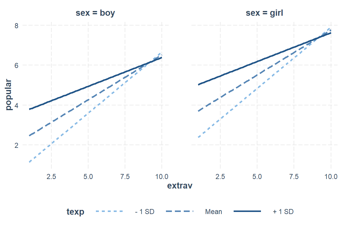

interactions::sim_slopes(model = pop_lmer_2_re,
                         pred = extrav,
                         modx = texp)

JOHNSON-NEYMAN INTERVAL

When texp is OUTSIDE the interval [29.16, 37.41], the slope of extrav is p
< .05.

Note: The range of observed values of texp is [2.00, 25.00]

SIMPLE SLOPES ANALYSIS

Slope of extrav when texp =  7.711184 (- 1 SD): 

  Est.   S.E.   t val.      p
------ ------ -------- ------
  0.61   0.02    25.59   0.00

Slope of extrav when texp = 14.263000 (Mean): 

  Est.   S.E.   t val.      p
------ ------ -------- ------
  0.45   0.02    25.89   0.00

Slope of extrav when texp = 20.814816 (+ 1 SD): 

  Est.   S.E.   t val.      p
------ ------ -------- ------
  0.29   0.02    11.86   0.00

For student’s who’s teach has average experience (M = 14.25 years), a 1 unit increase in extraversion is associated with a nearly half point increase in popularity, b = 0.45, SE = 0.02, p < .01. When the teacher has more experience, this association is less distinct and when teachers have more experience, this relationship is more pronounced.

Girls have higher popularities after controlling for their level of extroversion and their teacher’s experience, b = 1.24, SE = 0.04, p < .001.

interactions::sim_slopes(model = pop_lmer_2_re,
                         pred = extrav,
                         modx = texp,
                         modx.values = c(5, 10, 20))

JOHNSON-NEYMAN INTERVAL

When texp is OUTSIDE the interval [29.16, 37.41], the slope of extrav is p
< .05.

Note: The range of observed values of texp is [2.00, 25.00]

SIMPLE SLOPES ANALYSIS

Slope of extrav when texp =  5.00: 

  Est.   S.E.   t val.      p
------ ------ -------- ------
  0.68   0.03    23.33   0.00

Slope of extrav when texp = 10.00: 

  Est.   S.E.   t val.      p
------ ------ -------- ------
  0.56   0.02    27.29   0.00

Slope of extrav when texp = 20.00: 

  Est.   S.E.   t val.      p
------ ------ -------- ------
  0.31   0.02    13.46   0.00

For publications, you can get fancier

interactions::interact_plot(pop_lmer_2_re,                # model name
                            pred = extrav,                # x-axis 'predictor' variable name
                            modx = texp,                  # 'moderator' variable name
                            modx.values = c(5, 15, 25),   # values to pick for a continuous "modx"
                            interval = TRUE,              # adds CI bands for pop/marginal mean
                            y.label = "Estimated Marginal Mean\nPupil Popularity, Mean Rating of Classroom Peers",
                            x.label = "Pupil's Extroversion, as Rated by Teacher",
                            legend.main = "Teacher's Experience",
                            modx.labels = c("5 years",
                                            "15 years",
                                            "25 years"),
                            colors = c("black", "black", "black")) +   # default is "Blues" for modx.values
  theme_bw() +
  theme(legend.key.width = unit(2, "cm"),
        legend.background = element_rect(color = "Black"),
        legend.position = c(1, 0),
        legend.justification = c(1.1, -0.1)) +
  scale_x_continuous(breaks = seq(from = 0, to = 10, by = 2)) +
  scale_y_continuous(breaks = seq(from = 0, to = 10, by = 1))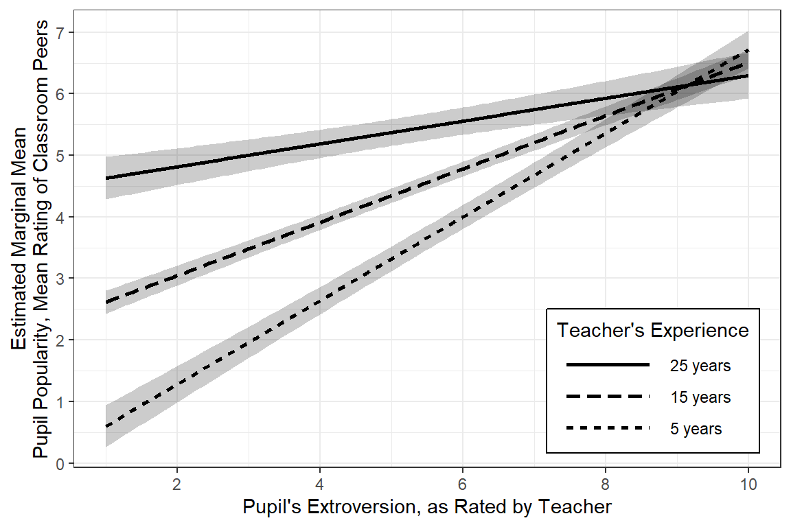

5.4.6.4 Visualization - `effects` & `ggplot2` packages

Get Estimated Marginal Means - default ‘nice’ predictor values:

Focal predictors: All combinations of… * sex categorical, both levels
* extrav continuous 1-10, default: 1, 3, 6, 8, 10
* texp continuous, default: 2.0, 7.8, 14.0, 19.0, 25.0

Always followed by: * fit estimated marginal mean * se standard error for the marginal mean * lower lower end of the 95% confidence interval around the estimated marginal mean * upper upper end of the 95% confidence interval around the estimated marginal mean

effects::Effect(focal.predictors = c("sex", "extrav", "texp"),
                mod = pop_lmer_2_re) %>% 
  data.frame() %>% 
  head(n = 12)

    sex extrav texp         fit        se      lower    upper
1   boy      1  2.0 -0.00309304 0.2113486 -0.4175801 0.411394
2  girl      1  2.0  1.23760458 0.2138348  0.8182417 1.656967
3   boy      3  2.0  1.50515155 0.1580364  1.1952179 1.815085
4  girl      3  2.0  2.74584917 0.1602463  2.4315815 3.060117
5   boy      6  2.0  3.76751843 0.1201262  3.5319324 4.003104
6  girl      6  2.0  5.00821605 0.1208433  4.7712237 5.245208
7   boy      8  2.0  5.27576302 0.1416431  4.9979792 5.553547
8  girl      8  2.0  6.51646064 0.1410030  6.2399322 6.792989
9   boy     10  2.0  6.78400761 0.1892756  6.4128090 7.155206
10 girl     10  2.0  8.02470523 0.1878580  7.6562868 8.393124
11  boy      1  7.8  1.16542895 0.1405371  0.8898140 1.441044
12 girl      1  7.8  2.40612657 0.1432221  2.1252460 2.687007

Pick ‘nicer’ illustrative values for texp

effects::Effect(focal.predictors = c("sex", "extrav", "texp"),
                mod = pop_lmer_2_re,
                xlevels = list(texp = c(5, 15, 25))) %>% 
  data.frame() %>% 
  head(n = 12)

    sex extrav texp       fit         se     lower     upper
1   boy      1    5 0.6013149 0.17312220 0.2617956 0.9408341
2  girl      1    5 1.8420125 0.17571483 1.4974087 2.1866163
3   boy      3    5 1.9611907 0.12951144 1.7071988 2.2151826
4  girl      3    5 3.2018883 0.13176041 2.9434859 3.4602908
5   boy      6    5 4.0010044 0.09857020 3.8076931 4.1943158
6  girl      6    5 5.2417021 0.09913857 5.0472761 5.4361281
7   boy      8    5 5.3608803 0.11620954 5.1329755 5.5887850
8  girl      8    5 6.6015779 0.11532656 6.3754048 6.8277510
9   boy     10    5 6.7207561 0.15520274 6.4163796 7.0251325
10 girl     10    5 7.9614537 0.15351429 7.6603886 8.2625189
11  boy      1   15 2.6160080 0.09471492 2.4302574 2.8017585
12 girl      1   15 3.8567056 0.09677976 3.6669056 4.0465056

Basic, default plot

Other than selecting three illustrative values for the teacher extroversion rating, most everything is left to default.

effects::Effect(focal.predictors = c("sex", "extrav", "texp"),
                mod = pop_lmer_2_re,
                xlevels = list(texp = c(5, 15, 25))) %>% 
  data.frame() %>% 
  dplyr::mutate(texp = factor(texp)) %>% 
  ggplot() +
  aes(x = extrav,
      y = fit,
      fill = texp,
      linetype = texp) +
  geom_ribbon(aes(ymin = lower,
                  ymax = upper),
              alpha = .3) +
  geom_line(aes(color = texp)) +
  facet_grid(.~ sex)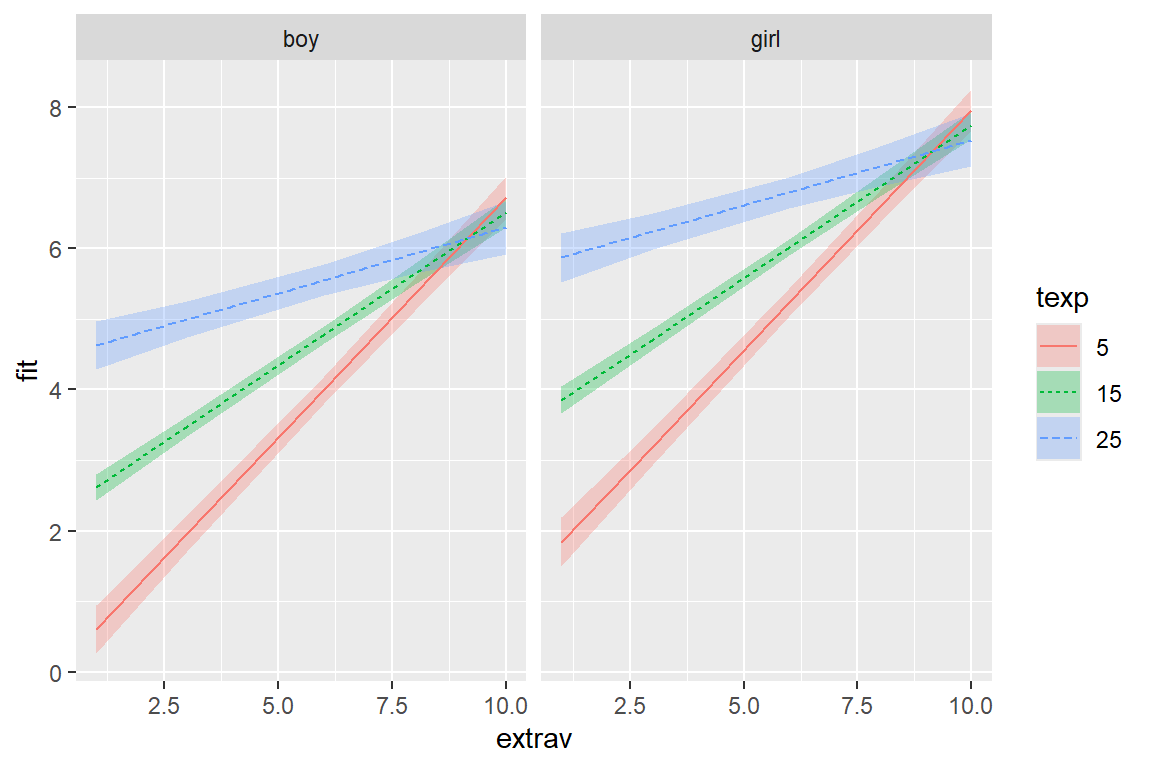

More Clean Plot

There are many ways to clean up a plot, including labeling the axes.

effects::Effect(focal.predictors = c("sex", "extrav", "texp"),
                mod = pop_lmer_2_re,
                xlevels = list(texp = c(5, 15, 25))) %>% 
  data.frame() %>% 
  dplyr::mutate(texp = factor(texp)) %>% 
  dplyr::mutate(sex = sex %>% 
                  forcats::fct_recode("Amoung Boys" = "boy",
                                      "Among Girls" = "girl")) %>% 
  ggplot() +
  aes(x = extrav,
      y = fit,
      fill = texp,
      linetype = texp) +
  geom_ribbon(aes(ymin = lower,
                  ymax = upper),
              alpha = .3) +
  geom_line(aes(color = texp)) +
  theme_bw() +
  facet_grid(.~ sex) +
  labs(x = "Pupil's Extroversion, Rated by Teacher",
       y = "Estimated Marginal Mean\nPupil Popularity, Mean Rating of Classroom Peers",
       color    = "Teacher's Experience, Years",
       linetype = "Teacher's Experience, Years",
       fill     = "Teacher's Experience, Years") +
  theme(legend.position = "bottom") +
  scale_x_continuous(breaks = seq(from = 0, to = 10, by = 2))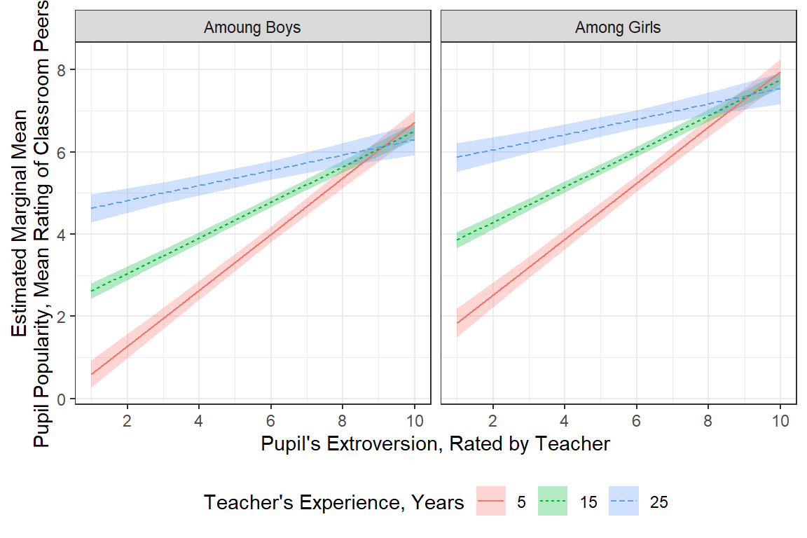

Publishable Plot

Since gender only exhibited a main effect and is not involved in any interactions, if would be a better use of space to not muddy the water with seperate panels. The Effect() function will estimate the marginal means using the reference category for categorical variables and the mean for continuous variables.

effects::Effect(focal.predictors = c("extrav", "texp"),  # choose not to investigate sex (the reference category will be used)
                mod = pop_lmer_2_re,
                xlevels = list(texp = c(5, 15, 25))) %>% 
  data.frame() %>% 
  dplyr::mutate(texp = factor(texp) %>% 
                  forcats::fct_rev()) %>% 
  ggplot() +
  aes(x = extrav,
      y = fit,
      linetype = texp) +
  geom_ribbon(aes(ymin = lower,
                  ymax = upper),
              fill = "black",
              alpha = .3) +
  geom_line() +
  theme_bw() +
  labs(x = "Pupil's Extroversion, Rated by Teacher",
       y = "Estimated Marginal Mean\nPupil Popularity, Mean Rating of Classroom Peers",
       color    = "Teacher's\nExperience,\nYears",
       linetype = "Teacher's\nExperience,\nYears",
       alpha    = "Teacher's\nExperience,\nYears") +
  theme(legend.key.width = unit(2, "cm"),
        legend.background = element_rect(color = "Black"),
        legend.position = c(1, 0),
        legend.justification = c(1.1, -0.1)) +
  scale_linetype_manual(values = c("solid", "dashed", "dotted")) +
  scale_x_continuous(breaks = seq(from = 0, to = 10, by = 2)) +
  scale_y_continuous(breaks = seq(from = 0, to = 10, by = 1))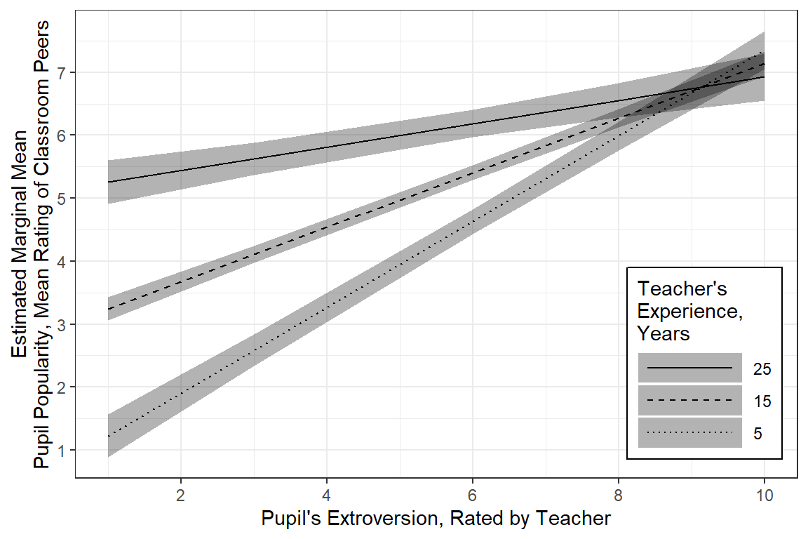

5.4.6.5 Interpretation

After accounting for class-to-class variation and the effect of gender, a positive association was found between teacher rated extroversion and peer rated popularity. This relationship was more marked for less experienced teachers.

5.4.7 Residual Plots

Form more infromation, see the vingette page for the redre package.

sjPlot::plot_model(pop_lmer_2_re,
                   type = "diag")

[[1]]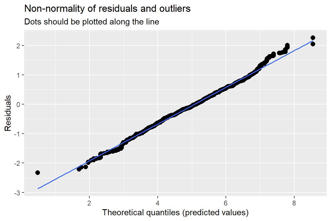


[[2]]
[[2]]$class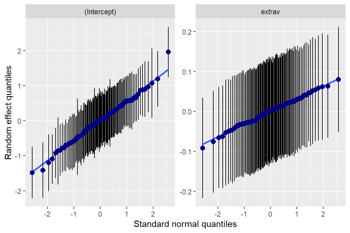



[[3]]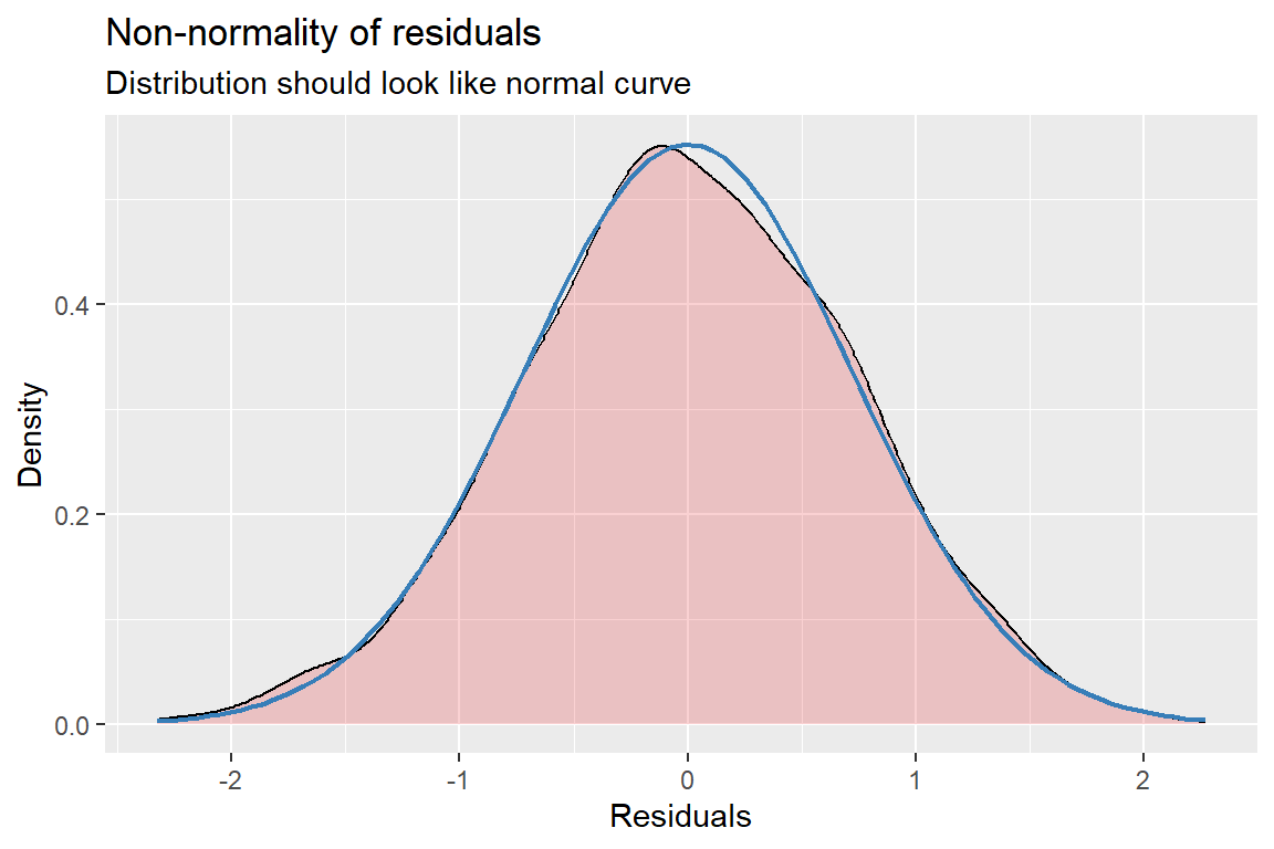


[[4]]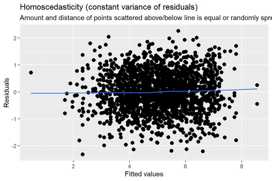

Standardized residuals vs. fitted values

You always want to use studentized, conditional residuals for MLM!

As you look across the plot, left to right:

GOOD = no pattern & HOV
BAD = any pattern or change in the spread

This plot looks great!

Type	Parameter of Interest	Estimates This
Fixed	Intercept	\(\beta_{0}\)
Random	Residual Variance \(var[e_{ij}]\)	\(\sigma^2_{e}\)

Type	Parameter of Interest	Estimates This
Fixed	Intercept	\(\gamma_{00}\)
Random	Variance in random intercepts, \(var[u_{0j}]\)	\(\sigma^2_{u0}\)
Random	Residual Variance \(var[e_{ij}]\)	\(\sigma^2_{e}\)