12 MLM, Longitudinal: Hedeker & Gibbons - Depression

install.packages("devtools")
devtools::install_github("sarbearschwartz/apaSupp") # updated 9/17/2025

Load/activate these packages

library(HLMdiag)      # package with the dataset
library(tidyverse)    
library(flextable)
library(apaSupp)      # Not on CRAN, on GitHub (see above)
library(psych)
library(VIM)         
library(naniar) 
library(lme4)        
library(lmerTest)
library(optimx)
library(performance)
library(interactions)
library(emmeans)
library(ggResidpanel)
library(HLMdiag)
library(sjPlot)


library(sjstats)      # ICC calculations
library(effects)      # Estimated Marginal Means

library(corrplot)     # Visualize correlation matrix

12.1 Background

Starting in chapter 4, (Hedeker and Gibbons 2006) details analysis of a psychiatric study described by (Reisby et al. 1977). This study focuses on the relationship between Imipramine (IMI) and Desipramine (DMI) plasma levels and clinical response in 66 depressed inpatients (37 endogenous and 29 non-endogenous).

Note: The IMI and DMI measures were only taken in the later weeks, but are not used here.

hamd Hamilton Depression Scores (HD)

Independent or predictor variables:

endog Depression Diagnosis
endogenous
non-endogenous/reactive
IMI (imipramine) drug-plasma levels (µg/l)
antidepressant given 225 mg/day, weeks 3-6
DMI (desipramine) drug-plasma levels (µg/l)
metabolite of imipramine

data_raw <- read.table("data/riesby.dat.txt") %>% 
  dplyr::rename(id    = "V1",
                hamd  = "V2",
                endog = "V5",
                week  = "V4") %>%
  dplyr::select(-V3, -V6)

data_raw %>% 
  psych::headTail(top = 11, bottom = 8)

     id hamd week endog
1   101   26    0     0
2   101   22    1     0
3   101   18    2     0
4   101    7    3     0
5   101    4    4     0
6   101    3    5     0
7   103   33    0     0
8   103   24    1     0
9   103   15    2     0
10  103   24    3     0
11  103   15    4     0
... ... <NA>  ...   ...
389 360   28    4     1
390 360   33    5     1
391 361   30    0     1
392 361   22    1     1
393 361   11    2     1
394 361    8    3     1
395 361    7    4     1
396 361   19    5     1

12.1.1 Long Format

data_long <- data_raw %>%                        
  dplyr::filter(!is.na(hamd)) %>%                                # remove NA or missing scores
  dplyr::mutate(id = factor(id)) %>%                             # declare grouping var a factor
  dplyr::mutate(endog = factor(endog,                            # attach labels to a grouping variable
                               levels = c(0, 1),                 # order of the levels should match levels
                               labels = c("Reactive",            # order matters!
                                          "Endogenous"))) %>% 
  dplyr::mutate(hamd = as.numeric(hamd)) %>% 
  dplyr::select(id, week, endog, hamd) %>%                       # select the order of variables to include
  dplyr::arrange(id, week)                                       # sort observations

data_long %>% 
  psych::headTail(top = 11, bottom = 8)

      id week      endog hamd
1    101    0   Reactive   26
2    101    1   Reactive   22
3    101    2   Reactive   18
4    101    3   Reactive    7
5    101    4   Reactive    4
6    101    5   Reactive    3
7    103    0   Reactive   33
8    103    1   Reactive   24
9    103    2   Reactive   15
10   103    3   Reactive   24
11   103    4   Reactive   15
... <NA>  ...       <NA>  ...
389  609    4 Endogenous   15
390  609    5 Endogenous    2
391  610    0 Endogenous   34
392  610    1 Endogenous <NA>
393  610    2 Endogenous   33
394  610    3 Endogenous   23
395  610    4 Endogenous <NA>
396  610    5 Endogenous   11

12.1.2 Wide Format

data_wide <- data_long %>%     # save the dataset as a new name
  tidyr::pivot_wider(names_from = week,
                     names_prefix = "hamd_",
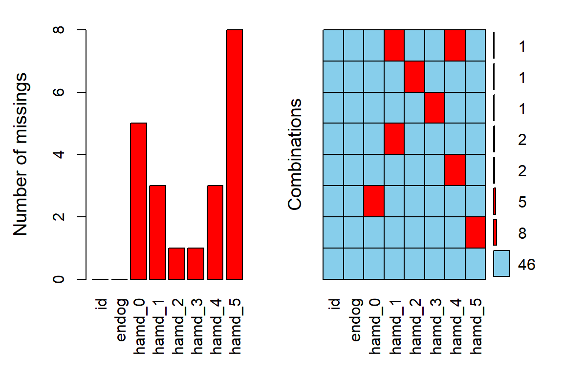
                     values_from = hamd)

Notice the missing values, displayed as NA.

data_wide %>% 
  psych::headTail()

    id      endog hamd_0 hamd_1 hamd_2 hamd_3 hamd_4 hamd_5
1  101   Reactive     26     22     18      7      4      3
2  103   Reactive     33     24     15     24     15     13
3  104 Endogenous     29     22     18     13     19      0
4  105   Reactive     22     12     16     16     13      9
5 <NA>       <NA>    ...    ...    ...    ...    ...    ...
6  607 Endogenous     30     39     30     27     20      4
7  608   Reactive     24     19     14     12      3      4
8  609 Endogenous   <NA>     25     22     14     15      2
9  610 Endogenous     34   <NA>     33     23   <NA>     11

12.2 Exploratory Data Analysis

12.2.1 Diagnosis Group

data_wide %>% 
  dplyr::select("Depression Type" = endog) %>% 
  apaSupp::tab_freq()

**Table 12.1**
Summary of Categorical Variables
		Statistic (N=66)
Depression Type
Reactive		29 (43.9%)
Endogenous		37 (56.1%)

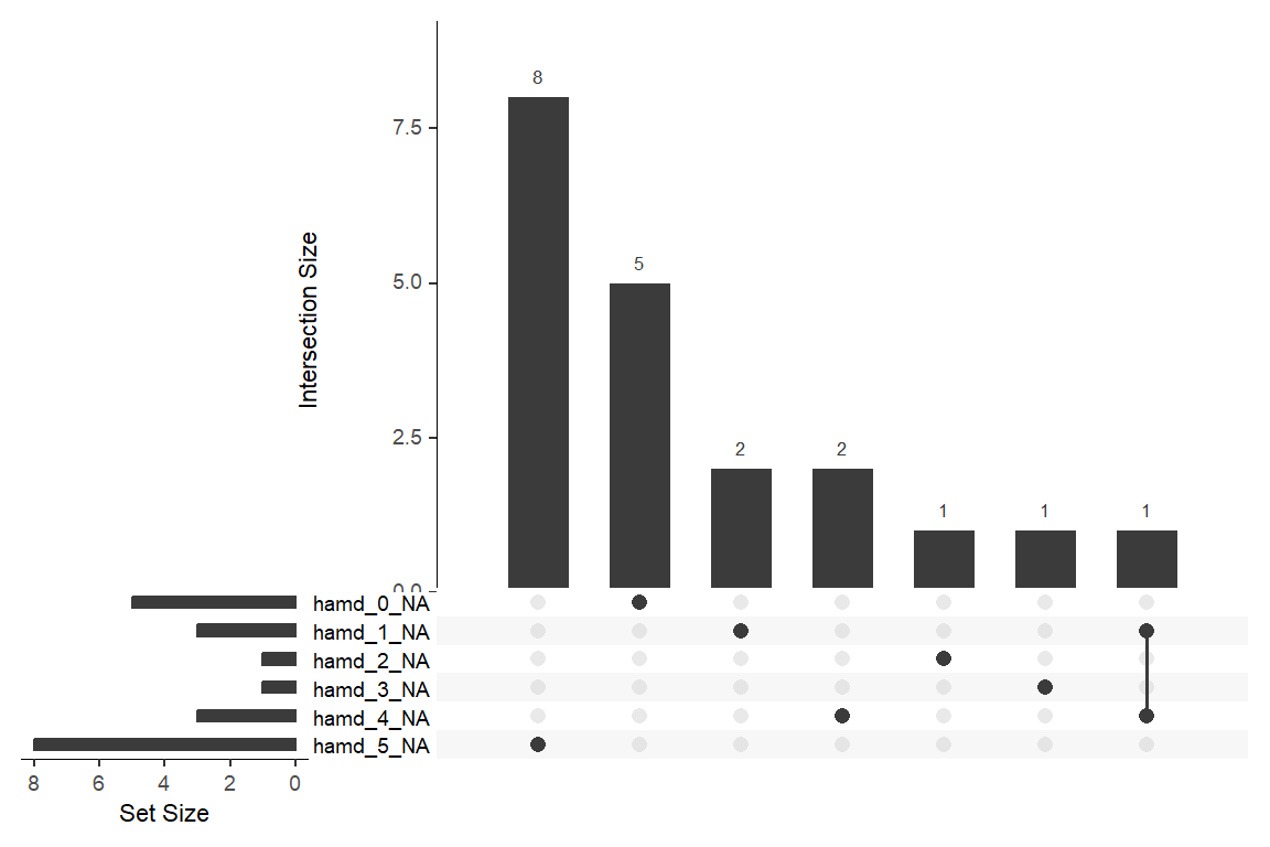
12.2.2 Missing Data & Attrition

Plot the amount of missing values and the amount of each patter of missing values.

12.2.2.1 `VIM` package

data_wide %>% 
  VIM::aggr(numbers = TRUE,   # shows the number to the far right
            prop = FALSE)     # shows counts instead of proportions

12.2.2.2 `naniar` package

data_wide %>% 
  naniar::gg_miss_upset(sets = c("hamd_5_NA",
                                 "hamd_4_NA",
                                 "hamd_3_NA",
                                 "hamd_2_NA",
                                 "hamd_1_NA",
                                 "hamd_0_NA"),
                        keep.order = TRUE)

12.2.3 Depression Over Time, by Group

12.2.3.1 Table of Means

data_wide %>%          
  dplyr::select(endog,
                "Baseline" = hamd_0,
                "Week 1" = hamd_1,
                "Week 2" = hamd_2,
                "Week 3" = hamd_3,
                "Week 4" = hamd_4,
                "Week 5" = hamd_5) %>% 
  apaSupp::tab1(split = "endog",
                caption = "Hamilton Depression Scores Across Time, by Depression Type")

**Table 12.2**
Hamilton Depression Scores Across Time, by Depression Type
	Total N = 66	Reactive n = 29 (43.9%)	Endogenous n = 37 (56.1%)	p-value
Baseline	23.44 (4.53)	22.79 (4.12)	24.00 (4.85)	.295
Unknown	5	1	4
Week 1	21.84 (4.70)	20.48 (3.83)	23.00 (5.10)	.029*
Unknown	3	0	3
Week 2	18.31 (5.49)	17.00 (4.35)	19.30 (6.08)	.081
Unknown	1	1	0
Week 3	16.42 (6.42)	15.34 (6.17)	17.28 (6.56)	.227
Unknown	1	0	1
Week 4	13.62 (6.97)	12.62 (6.72)	14.47 (7.17)	.295
Unknown	3	0	3
Week 5	11.95 (7.22)	11.22 (6.34)	12.58 (7.96)	.473
Unknown	8	2	6
Note. Continuous variables are summarized with means (SD) and significant group differences assessed via independent t-tests. Categorical variables are summarized with counts (%) and significant group differences assessed via Chi-squared tests for independence.
* p < .05. p < .01. * p < .001.

12.2.3.2 Using the LONG formatted dataset

Each person’s data is stored on multiple lines, one for each time point.

FOR ALL DATA AVAILABLE!

data_long %>% 
  dplyr::group_by(endog, week) %>%                # specify the groups
  dplyr::filter(!is.na(hamd)) %>% 
  dplyr::summarise(hamd_n    = n(),                      # count of valid scores
                   hamd_mean = mean(hamd),               # mean score
                   hamd_sd   = sd(hamd),                 # standard deviation of scores
                   hamd_sem  = hamd_sd / sqrt(hamd_n)) %>%  # stadard error for the mean of scores 
  flextable::as_grouped_data(groups = "endog") %>% 
  flextable::flextable() %>% 
  flextable::separate_header() %>% 
  apaSupp::theme_apa() %>% 
  flextable::hline(part = "header", i = 1)

**Table 12.3**
Table Caption
endog	week	hamd
endog	week	n	mean	sd	sem
Reactive
	0	28	22.79	4.12	0.78
	1	29	20.48	3.83	0.71
	2	28	17.00	4.35	0.82
	3	29	15.34	6.17	1.15
	4	29	12.62	6.72	1.25
	5	27	11.22	6.34	1.22
Endogenous
	0	33	24.00	4.85	0.84
	1	34	23.00	5.10	0.87
	2	37	19.30	6.08	1.00
	3	36	17.28	6.56	1.09
	4	34	14.47	7.17	1.23
	5	31	12.58	7.96	1.43

FOR COMPLETE CASES ONLY!!!

data_long %>% 
  dplyr::group_by(id) %>%               # group-by participant
  dplyr::filter(!is.na(hamd)) %>% 
  dplyr::mutate(person_vsae_n = n()) %>%    # count the number of valid VSAE scores
  dplyr::filter(person_vsae_n == 6) %>%     # restrict to only thoes children with 5 valid scores
  dplyr::group_by(endog, week) %>%                # specify the groups
  dplyr::summarise(hamd_n    = n(),                      # count of valid scores
                   hamd_mean = mean(hamd),               # mean score
                   hamd_sd   = sd(hamd),                 # standard deviation of scores
                   hamd_sem  = hamd_sd / sqrt(hamd_n)) %>%  # stadard error for the mean of scores 
  flextable::as_grouped_data(groups = "endog") %>% 
  flextable::flextable() %>% 
  flextable::separate_header() %>% 
  apaSupp::theme_apa() %>% 
  flextable::hline(part = "header", i = 1)

**Table 12.4**
Table Caption
endog	week	hamd
endog	week	n	mean	sd	sem
Reactive
	0	25	22.36	3.90	0.78
	1	25	20.08	3.68	0.74
	2	25	17.32	4.34	0.87
	3	25	15.88	5.84	1.17
	4	25	12.84	6.68	1.34
	5	25	11.40	6.54	1.31
Endogenous
	0	21	24.10	4.87	1.06
	1	21	23.90	5.47	1.19
	2	21	18.95	6.01	1.31
	3	21	17.48	6.86	1.50
	4	21	14.19	6.98	1.52
	5	21	13.05	8.73	1.90

12.2.3.3 Person-Profile Plot or Spaghetti Plot

Use the data in LONG format.

A scatterplot of all observations of depression scores over time, joining the dots of each individual’s data.

NOTE: Not all lines have a point for every week!

data_long %>% 
  dplyr::filter(!is.na(hamd)) %>% 
  ggplot(aes(x = week,
             y = hamd)) +
  geom_point() +
  geom_line(aes(group = id)) +   # join points that belong to the same "id"
  theme_bw() +
  labs(x = "Weeks Since Baseline",
       y = "Estimated Hamilton Depression Score (HD)")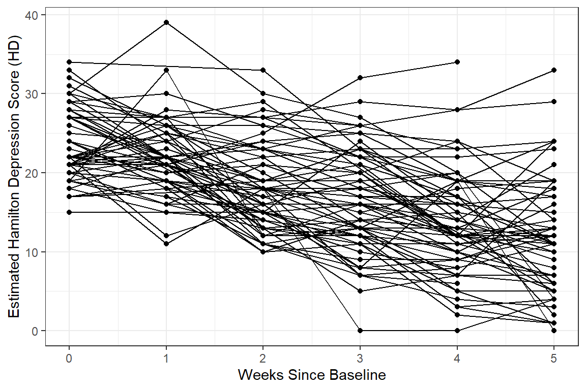

data_long %>% 
  dplyr::filter(!is.na(hamd)) %>% 
  ggplot(aes(x = week,
             y = hamd,
             color = endog)) +    # color points and lines by the "endog" variable
  geom_line(aes(group = id)) +
  theme_bw() +
  labs(x = "Weeks Since Baseline",
       y = "Estimated Hamilton Depression Score (HD)")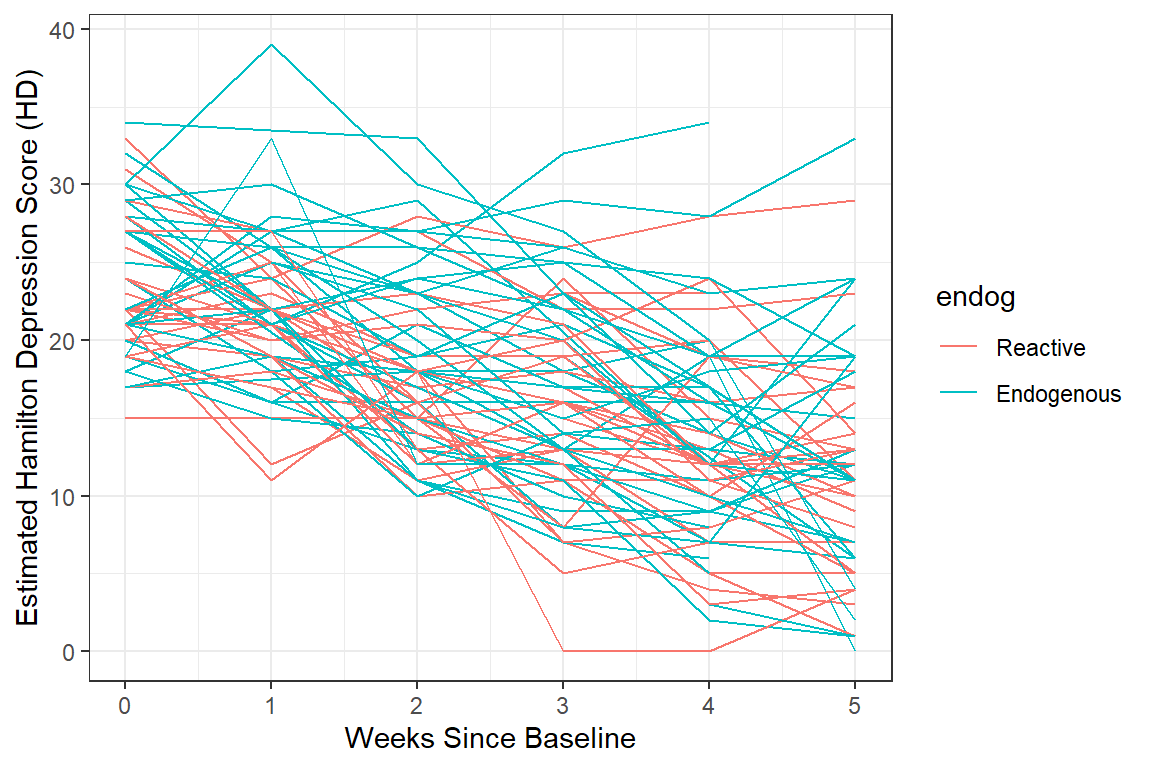

data_long %>% 
  dplyr::filter(!is.na(hamd)) %>% 
  ggplot(aes(x = week,
             y = hamd)) +
  geom_line(aes(group = id)) +
  facet_grid( ~ endog) +           # side-by-side pandels by the "endog" variable
  theme_bw() +
  labs(x = "Weeks Since Baseline",
       y = "Estimated Hamilton Depression Score (HD)")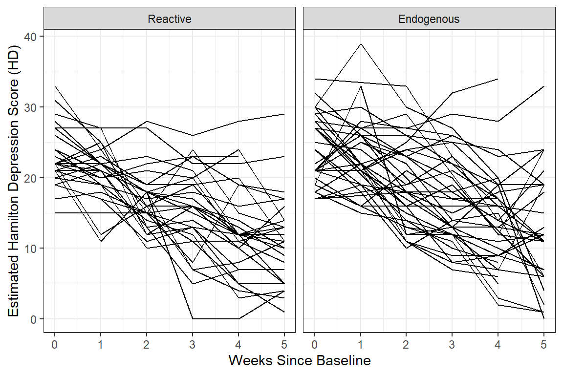

data_long %>% 
  dplyr::filter(!is.na(hamd)) %>% 
  ggplot(aes(x = week %>% factor(),
             y = hamd)) +
  geom_boxplot() +                   # compare center and spread
  facet_grid( ~ endog) +  
  theme_bw() +
  labs(x = "Weeks Since Baseline",
       y = "Estimated Hamilton Depression Score (HD)")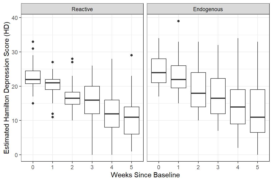

data_long %>% 
  dplyr::filter(!is.na(hamd)) %>% 
  ggplot(aes(x = week %>% factor(),
             y = hamd)) +
  geom_violin(fill = "gray75") +                   # similar to boxplots to show distribution
  stat_summary() +  
  stat_summary(aes(group = "endog"),
               fun = mean,
               geom = "line") +
  facet_grid( ~ endog)   +  
  theme_bw() +
  labs(x = "Weeks Since Baseline",
       y = "Estimated Hamilton Depression Score (HD)")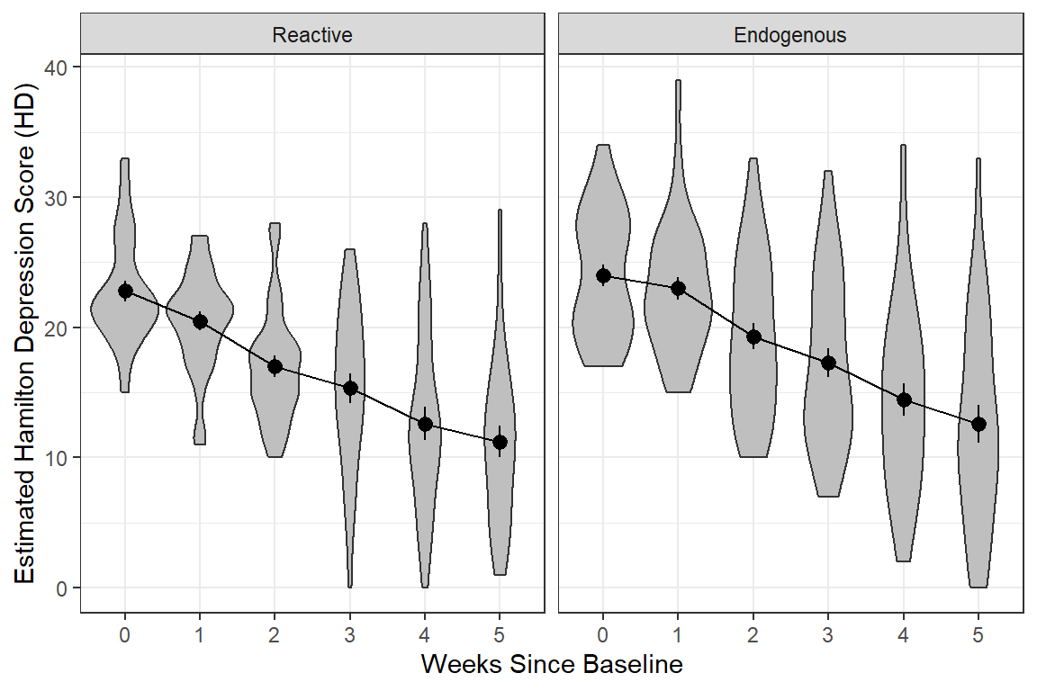

data_long %>% 
  dplyr::filter(!is.na(hamd)) %>% 
  ggplot(aes(x = week,
             y = hamd,
             color = endog)) +
  stat_summary() +
  stat_summary(aes(group = endog,
                   linetype = endog),
               fun = mean,
               geom = "line") +
  scale_linetype_manual(values = c("solid", "longdash")) +
  theme(legend.position = "bottom",
        legend.key.width = unit(2, "cm")) +  
  theme_bw() +
  labs(x = "Weeks Since Baseline",
       y = "Estimated Hamilton Depression Score (HD)")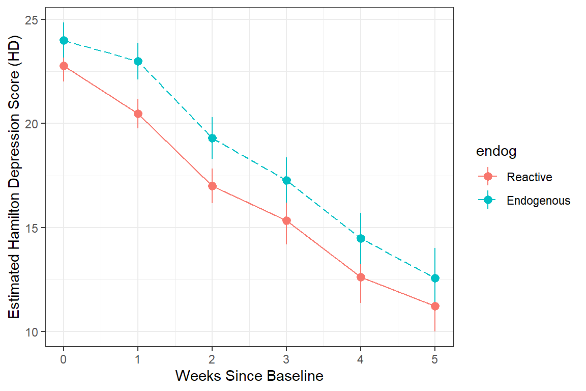

data_long %>% 
  dplyr::filter(!is.na(hamd)) %>% 
  ggplot(aes(x = week,
             y = hamd)) +
  geom_line(aes(group = id)) +
  facet_grid( ~ endog) +
  geom_smooth() +                     # DEFAULTS: method = "loess", se = TRUE, color = "blue"
  geom_smooth(method = "lm",
              se = FALSE,
              color = "hot pink")+  
  theme_bw() +
  labs(x = "Weeks Since Baseline",
       y = "Estimated Hamilton Depression Score (HD)")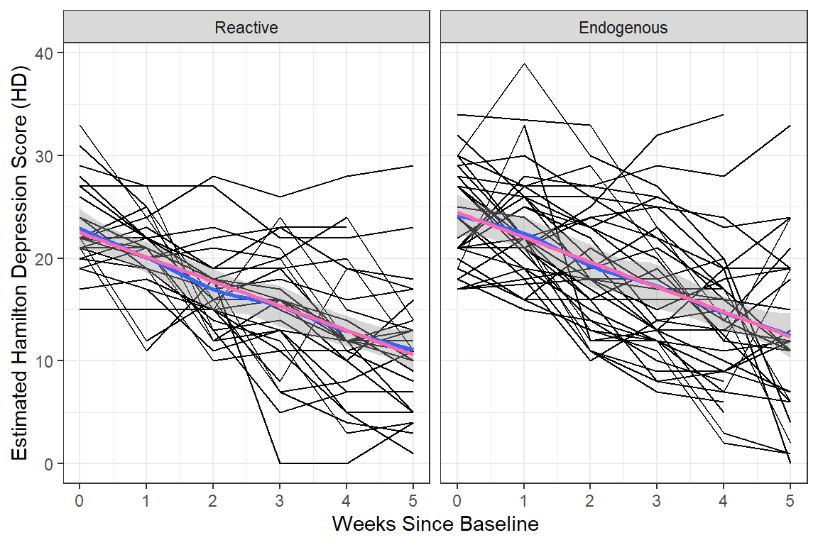

data_long %>% 
  dplyr::filter(!is.na(hamd)) %>% 
  ggplot(aes(x = week,
             y = hamd)) +
  facet_grid( ~ endog) +
  geom_smooth(aes(color = "Flexible"),
              method = "loess",
              se = FALSE,) +
  geom_smooth(aes(color = "Linear"),
              method = "lm",
              se = FALSE) +
  scale_color_manual(name = "Smoother Type: ",
                     values = c("Flexible" = "blue", 
                                "Linear"   = "red")) +
  theme_bw() + 
  theme(legend.position = "bottom") +
  labs(x = "Weeks Since Baseline",
       y = "Estimated Hamilton Depression Score (HD)")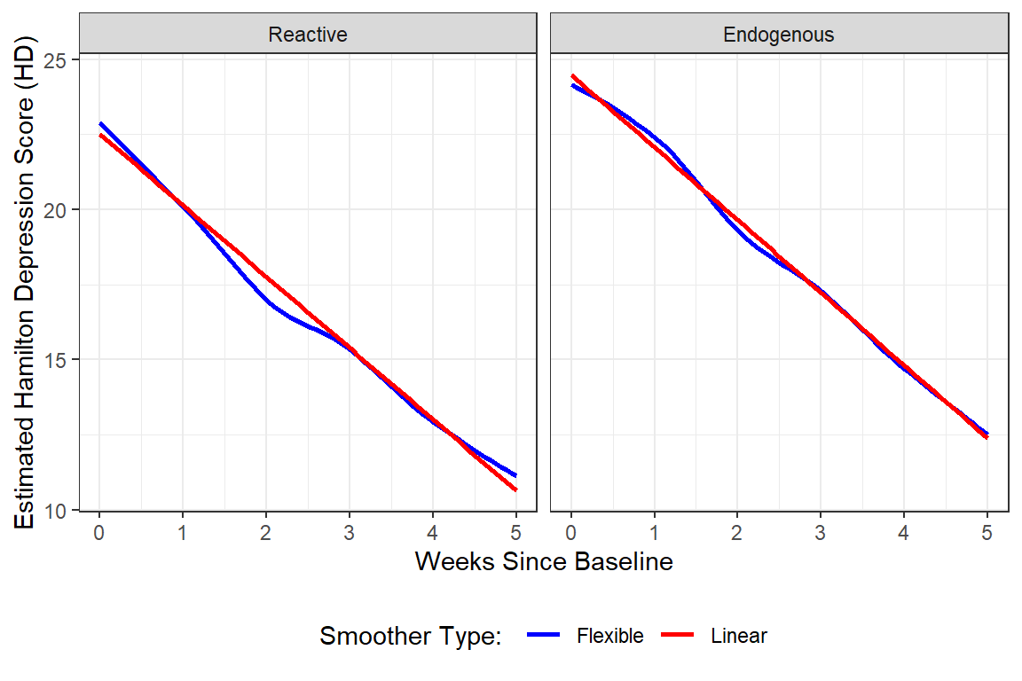

data_long %>% 
  ggplot(aes(x = week,
             y = hamd,
             group = endog,
             linetype = endog)) +
  geom_smooth(method = "loess",
              color = "black",
              alpha = .25) +
  theme_bw() +
  scale_linetype_manual(values = c("solid", "longdash")) +
  theme(legend.position = c(1, 1),
        legend.justification = c(1.1, 1.1),
        legend.background = element_rect(color = "black"),
        legend.key.width = unit(1.5, "cm")) +
  labs(x = "Weeks Since Baseline",
       y = "Estimated Hamilton Depression Scale",
       linetype = "Type of Depression")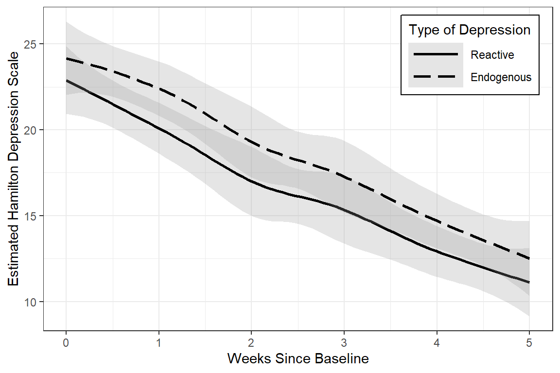

data_long %>% 
  dplyr::filter(!is.na(hamd)) %>% 
  ggplot(aes(x = week,
             y = hamd,
             group = endog,
             linetype = endog)) +
  geom_smooth(method = "loess",
              color = "black",
              alpha = .25) +
  theme_bw() +
  scale_linetype_manual(values = c("solid", "longdash")) +
  theme(legend.position = c(1, 1),
        legend.justification = c(1.1, 1.1),
        legend.background = element_rect(color = "black"),
        legend.key.width = unit(2, "cm")) +
  labs(x = "Weeks Since Baseline",
       y = "EsStimated Hamilton Depression Scale",
       linetype = "Type of Depression")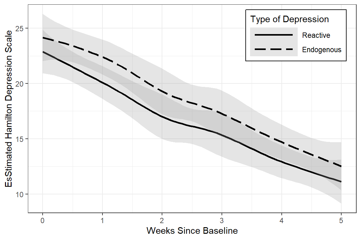

data_long %>% 
  dplyr::filter(!is.na(hamd)) %>% 
  ggplot(aes(x = week,
             y = hamd,
             group = endog,
             linetype = endog)) +
  geom_smooth(method = "lm",
              color = "black",
              alpha = .25) +
  theme_bw() +
  scale_linetype_manual(values = c("solid", "longdash")) +
  theme(legend.position = c(1, 1),
        legend.justification = c(1.1, 1.1),
        legend.background = element_rect(color = "black"),
        legend.key.width = unit(1.5, "cm")) +
  labs(x = "Weeks Since Baseline",
       y = "EStimated Hamilton Depression Scale",
       linetype = "Type of Depression")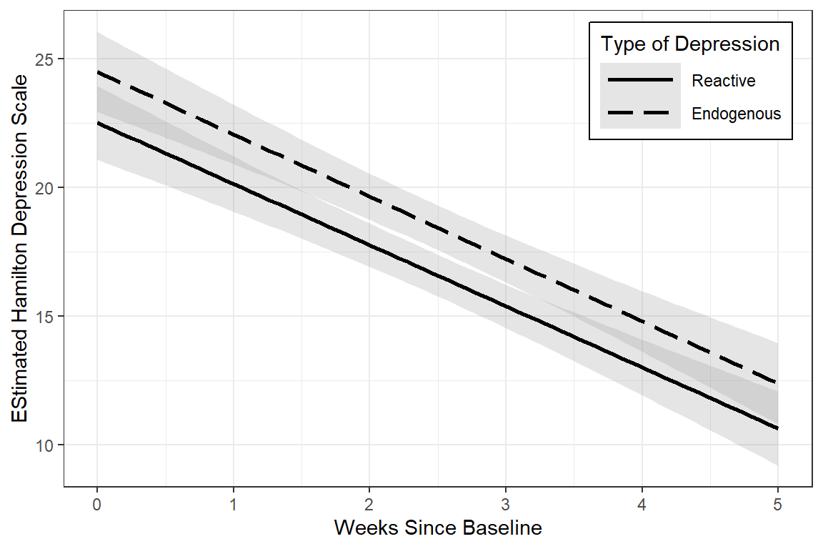

12.3 Patterns in the Outcome Over Time

12.3.1 Variance-Covariance

12.3.1.1 Full Matrix

Variances are down the diagonal
Increasing variance over time violates the ANOVA assumption of homogeity of variance

data_wide %>% 
  dplyr::select(starts_with("hamd_")) %>%  # just the outcome(s)
  cov(use = "complete.obs")  %>%           # covariance matrix, LIST-wise deletion
  round(3)

       hamd_0 hamd_1 hamd_2 hamd_3 hamd_4 hamd_5
hamd_0 19.421 10.716  9.523 12.350  9.062  7.376
hamd_1 10.716 24.236 12.545 15.930 11.592  8.471
hamd_2  9.523 12.545 26.773 23.848 23.858 20.657
hamd_3 12.350 15.930 23.848 39.755 33.316 29.728
hamd_4  9.062 11.592 23.858 33.316 45.943 37.107
hamd_5  7.376  8.471 20.657 29.728 37.107 57.332

data_wide %>% 
  dplyr::select(starts_with("hamd_")) %>%  # just the outcome(s)
  cov(use = "pairwise.complete.obs")  %>%  # covariance matrix, PAIR-wise deletion
  round(3)

       hamd_0 hamd_1 hamd_2 hamd_3 hamd_4 hamd_5
hamd_0 20.551 10.115 10.139 10.086  7.191  6.278
hamd_1 10.115 22.071 12.277 12.550 10.264  7.720
hamd_2 10.139 12.277 30.091 25.126 24.626 18.384
hamd_3 10.086 12.550 25.126 41.153 37.339 23.992
hamd_4  7.191 10.264 24.626 37.339 48.594 30.513
hamd_5  6.278  7.720 18.384 23.992 30.513 52.120

12.3.1.2 Just Variances

Notice the variance in scores increases over time, which is seen in the side-by-side boxplots.

data_wide %>% 
  dplyr::select(starts_with("hamd_")) %>%  # just the outcome(s)
  cov(use = "pairwise.complete.obs")  %>%  # covariance matrix, PAIR-wise deletion
  diag()                                   #  extracts just the variances

  hamd_0   hamd_1   hamd_2   hamd_3   hamd_4   hamd_5 
20.55082 22.07117 30.09135 41.15288 48.59447 52.12008

12.3.2 Correlation

12.3.2.1 Full Matrix

Pairwise relationships are easier to eye-ball magnitude when presented as correlations, rather than covariances, due to the relative scale.

data_wide %>% 
  dplyr::select(starts_with("hamd_")) %>% # just the outcome(s)
  cor(use = "complete.obs") %>%           # correlation matrix - LIST-wise deletion
  round(2)

       hamd_0 hamd_1 hamd_2 hamd_3 hamd_4 hamd_5
hamd_0   1.00   0.49   0.42   0.44   0.30   0.22
hamd_1   0.49   1.00   0.49   0.51   0.35   0.23
hamd_2   0.42   0.49   1.00   0.73   0.68   0.53
hamd_3   0.44   0.51   0.73   1.00   0.78   0.62
hamd_4   0.30   0.35   0.68   0.78   1.00   0.72
hamd_5   0.22   0.23   0.53   0.62   0.72   1.00

data_wide %>% 
  dplyr::select(starts_with("hamd_")) %>% # just the outcome(s)
  cor(use = "pairwise.complete.obs") %>%   # correlation matrix - PAIR-wise deletion
  round(2)

       hamd_0 hamd_1 hamd_2 hamd_3 hamd_4 hamd_5
hamd_0   1.00   0.49   0.41   0.33   0.23   0.18
hamd_1   0.49   1.00   0.49   0.41   0.31   0.22
hamd_2   0.41   0.49   1.00   0.74   0.67   0.46
hamd_3   0.33   0.41   0.74   1.00   0.82   0.57
hamd_4   0.23   0.31   0.67   0.82   1.00   0.65
hamd_5   0.18   0.22   0.46   0.57   0.65   1.00

12.3.2.2 Visualization

Looking for patterns is always easier with a plot. All RM or mixed ANOVA assume sphericity or compound symmetry, meaning that all the correlations in the matrix would be the same. This is not the case for these data. Instead we see a classic pattern of corralary decay. Measures taken close in time, say 1 week apart, exhibit the highest degree of correlation. The farther apart in time that two measures are taken, the less correlated they are. Note that the adjacent measures become more highly correlated, too. This can be due to attrition; later time points having a smaller sample size.

data_wide %>% 
  dplyr::select(starts_with("hamd_")) %>% # just the outcome(s)
  cor(use = "pairwise.complete.obs") %>%   # correlation matrix
  corrplot::corrplot.mixed(upper = "ellipse")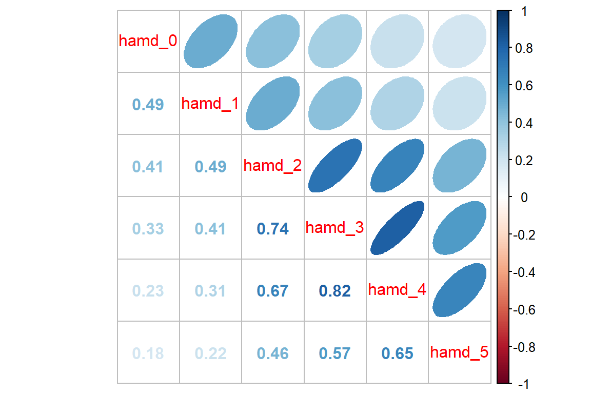

12.3.3 For Each Group

It can be a good ideal to investigate if the groups exhibit a similar pattern in correlation.

Reactive Depression

data_wide %>% 
  dplyr::filter(endog == "Reactive") %>%    # filter observations for the REACTIVE group
  dplyr::select(starts_with("hamd_")) %>% 
  cor(use = "pairwise.complete.obs") %>%   
  corrplot::corrplot.mixed(upper = "ellipse")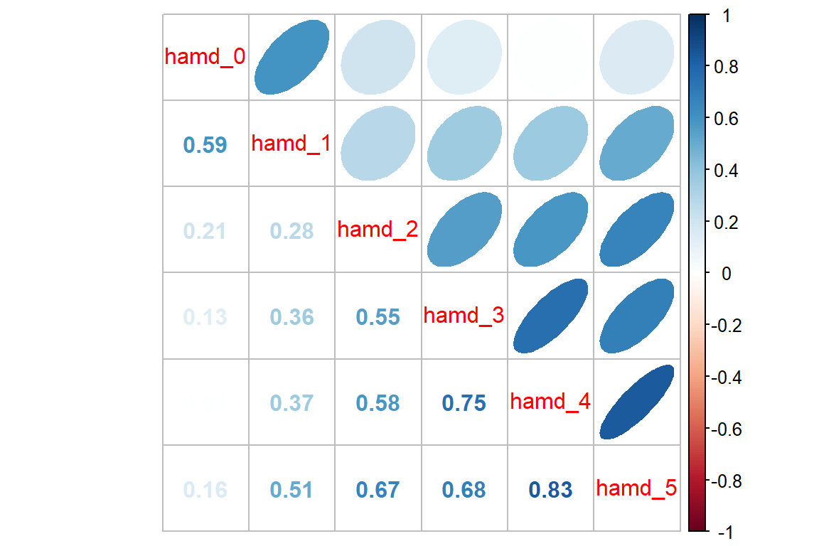

Endogenous Depression

data_wide %>% 
  dplyr::filter(endog == "Endogenous") %>%    # filter observations for the Endogenous group
  dplyr::select(starts_with("hamd_")) %>%
  cor(use = "pairwise.complete.obs") %>%   
  corrplot::corrplot.mixed(upper = "ellipse")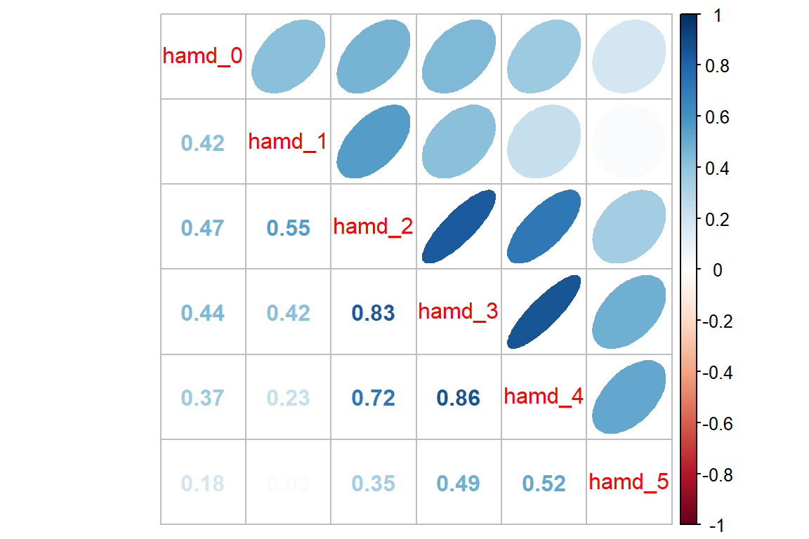

12.4 MLM - Null or Emptly Models

12.4.1 Fit the model

Random Intercepts, with Fixed Intercept and Time Slope (i.e. Trend)….@hedeker2006 section 4.3.5, starting on page 55

Since this situation deals with longitudinal data, it is more appropriate to start off including the time variable in the null model as a fixed effect only.

fit_lmer_week_RI_reml <- lmerTest::lmer(hamd ~ week + (1|id), 
                                        data = data_long,
                                        REML = TRUE)

12.4.2 Table of Parameter Estimates

apaSupp::tab_lmer(fit_lmer_week_RI_reml, 
                  caption = "MLM: Random Intercepts Null Model fit w/REML",
                  general_note = "Reproduction of Hedeker's table 4.3 on page 55, except using REML here instead of ML")

**Table 12.5**
MLM: Random Intercepts Null Model fit w/REML
	Est	(SE)	p
(Intercept)	23.55	(0.64)	< .001***
week	-2.38	(0.14)	< .001***
id.var__(Intercept)	16.45
Residual.var__Observation	19.10
Note. Est = estimated regresssion coefficient for fixed effects and varaince/covariance estimates for random effects. p = significance from Wald t-test for parameter estimate using Satterthwaite's method for degrees of freedom. Reproduction of Hedeker's table 4.3 on page 55, except using REML here instead of ML
* p < .05. p < .01. * p < .001.

On average, patients start off with HDRS scores of 23.55 and then change by -2.38 points each week. This weekly improvement of about 2 points a week is statistically significant via the Wald test.

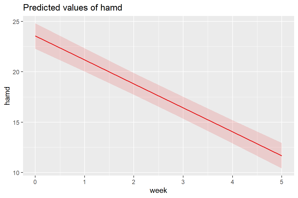
12.4.3 Estimated Marginal Means Plot

Multilevel model on page 55 (Hedeker and Gibbons 2006)

\[ \hat{y} = 23.552 + -2.376 week \]

The fastest way to plot a model is to use the sjPlot::plot_model() function.

Note: you can’t use interactions::interact_plot() since there is only one predictor (i.e. independent variable) in this model.

sjPlot::plot_model(fit_lmer_week_RI_reml,
                   type = "pred",
                   terms = c("week"))

12.4.4 Estimated Marginal Means and Emperical Bayes Plots

With a bit more code we can plot not only the marginal model (fixed effects only), but add the Best Linear Unbiased Predictions (BLUPs) or person-specific specific models (both fixed and random effects).

data_long %>% 
  dplyr::mutate(pred_fixed = predict(fit_lmer_week_RI_reml, 
                                     re.form = NA,           # fixed effects only
                                     newdata = .)) %>% 
  dplyr::mutate(pred_wrand = predict(fit_lmer_week_RI_reml,  # fixed and random effects both
                                     newdata = .)) %>%              
  ggplot(aes(x = week,
             y = hamd,
             group = id)) +
  geom_line(aes(y        = pred_wrand,
                color    = "BLUP",
                size     = "BLUP",
                linetype = "BLUP")) +
  geom_line(aes(y        = pred_fixed,
                color    = "Marginal",
                size     = "Marginal",
                linetype = "Marginal")) +
  theme_bw() +
  scale_color_manual(name   = "Type of Prediction",
                     values = c("BLUP"     = "gray50",
                                "Marginal" = "blue"))  +
  scale_size_manual(name    = "Type of Prediction",
                    values = c("BLUP"      = .5,
                               "Marginal" = 1.25))  +
  scale_linetype_manual(name   = "Type of Prediction",
                        values = c("BLUP"     = "longdash",
                                   "Marginal" = "solid"))  +
  theme(legend.position = c(0, 0),
        legend.justification = c(-0.1, -0.1),
        legend.background = element_rect(color = "black"),
        legend.key.width = unit(1.5, "cm")) +
  labs(x = "Weeks Since Baseline",
       y = "Estimated Hamilton Depression Score (HD)")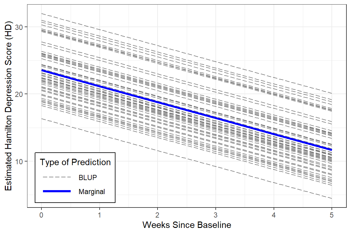

Notice that in this model, all the BLUPs are parallel. That is because we are only letting the intercept vary from person-to-person while keeping the effect of time (slope) constant.

Reproduce Table 4.4 on page 55 (Hedeker and Gibbons 2006)

One way to judge a model is to compare the estimated means to the observed means to see how accuratedly they are represented by the model. This excellent fit of the estimated marginal means to the observed data supports the hypothesis that the change in depression across time is LINEAR.

obs <- data_long %>% 
  dplyr::group_by(week) %>% 
  dplyr::summarise(observed = mean(hamd, na.rm = TRUE)) 

effects::Effect(focal.predictors = "week",
                mod = fit_lmer_week_RI_reml,
                xlevels = list(week = 0:5)) %>% 
  data.frame() %>% 
  dplyr::rename(estimated = fit) %>% 
  dplyr::left_join(obs, by = "week") %>% 
  dplyr::select(week, observed, estimated) %>% 
  dplyr::mutate(diff = observed - estimated) %>% 
  flextable::flextable() %>% 
  apaSupp::theme_apa(caption = "Observed and Estimated Means")

**Table 12.6**
Observed and Estimated Means
week	observed	estimated	diff
0.00	23.44	23.55	-0.11
1.00	21.84	21.18	0.67
2.00	18.31	18.80	-0.49
3.00	16.42	16.42	-0.01
4.00	13.62	14.05	-0.43
5.00	11.95	11.67	0.27

12.4.5 Intra-individual Correlation (ICC)

performance::icc(fit_lmer_week_RI_reml)

# Intraclass Correlation Coefficient

    Adjusted ICC: 0.463
  Unadjusted ICC: 0.319

Interpretation Just less than a third ($\rho_c = .32$) in baseline depression is explained by person-to-person differences. Thus, subjects display considerable heterogeneity in depression levels.

This value of .46is an oversimplification of the correlation matrix above and may be thought of as the expected correlation between two randomly drawn weeks for any given person.

performance::r2(fit_lmer_week_RI_reml)

# R2 for Mixed Models

  Conditional R2: 0.629
     Marginal R2: 0.310

Interpretation Linear growth accounts for 31% of the variance in Hamilton Depression Scores across the six weeks. Linear growth AND person-to-person differences account for a total 63% of this variance.

This value of 46% is an oversimplification of the correlation matrix above and may be thought of as the expected correlation between two randomly drawn weeks for any given person.

performance::r2(fit_lmer_week_RI_reml)

# R2 for Mixed Models

  Conditional R2: 0.629
     Marginal R2: 0.310

Note: The marginal $R^2$ considers only the variance of the fixed effects, while the conditional $R^2$ takes both the fixed and random effects into account. The random effect variances are actually the mean random effect variances, thus the $R^2$ value is also appropriate for mixed models with random slopes or nested random effects (see Johnson 2014).

Interpretation Linear growth accounts for 31% of the variance in Hamilton Depression Scores across the six weeks. Linear growth AND person-to-person differences account for a total 63% of this variance.

Note: The marginal R^2 considers only the variance of the fixed effects, while the conditional R^2 takes both the fixed and random effects into account. The random effect variances are actually the mean random effect variances, thus the R^2 value is also appropriate for mixed models with random slopes or nested random effects (see Johnson 2014).

12.4.6 Compare to the Single-Level Null: No Random Effects

Simple Linear Regression, (Hedeker and Gibbons 2006)

To compare, fit the single level regression model

fit_lm_week_ml <- lm(hamd ~ week,
                     data = data_long)

12.4.6.1 Table of Parameter Estimates

texreg::screenreg(list(fit_lm_week_ml, fit_lmer_week_RI_reml),
                  custom.model.names = c("Single-Level", "Multilevel"),
                  single.row = TRUE,
                  caption = "MLM: Longitudinal Null Models",
                  caption.above = TRUE,
                  custom.note = "The singel-level model treats are observations as being independent and unrelated to each other, even if they were made on the same person.")

=========================================================== Single-Level Multilevel
———————————————————– (Intercept) 23.60 (0.55) *** 23.55 (0.64) week -2.41 (0.18) -2.38 (0.14) *** ———————————————————– R^2 0.32
Adj. R^2 0.32
Num. obs. 375 375
AIC 2294.73
BIC 2310.43
Log Likelihood -1143.36
Num. groups: id 66
Var: id (Intercept) 16.45
Var: Residual 19.10
=========================================================== The singel-level model treats are observations as being independent and unrelated to each other, even if they were made on the same person.

For the multilevel model, the Wald tests indicated the fixed intercept is significant (no surprised that the depressions scores are not zero at baseline). More of note is the significance of the fixed effect of time. This signifies that depression scores are declining over time. On average, patients are improving (Hamilton Depression Scores get smaller) across time, by an average of 2.4’ish points a week.

For the multilevel model, the Wald tests indicated the fixed intercept is significant (no surprised that the depressions scores are not zero at baseline). More of note is the significance of the fixed effect of time. This signifies that depression scores are declining over time. On average, patients are improving (Hamilton Depression Scores get smaller) across time, by an average of 2.4’ish points a week.

12.4.6.2 Residual Variance

Note, the fixed estimates are very similar for the two models, but the standard errors are different. Additionally, whereas the single-level regression lumps all remaining variance together ($\sigma^2$), the multilevel model seperates it into within-subjects ($\sigma^2_{u0}$ or $\tau_{00}$) and between-subjects variance ($\sigma^2_{e}$ or $\sigma^2$).

sigma(fit_lm_week_ml)^2

[1] 35.3997

lme4::VarCorr(fit_lmer_week_RI_reml) %>% # in longitudinal data, a group of observations = a participant or person
  print(comp = c("Variance", "Std.Dev"))

 Groups   Name        Variance Std.Dev.
 id       (Intercept) 16.446   4.0554  
 Residual             19.099   4.3703

“One statistician’s error term is another’s career!”

(Hedeker and Gibbons 2006), page 56

12.5 MLM: Add Random Slope for Time (i.e. Trend)

12.5.1 Fit the Model

fit_lmer_week_RIAS_reml <- lmerTest::lmer(hamd ~ week + (week|id), #     MLM-RIAS
                                          data = data_long,
                                          REML = TRUE)

apaSupp::tab_lmers(list("Random Intercepts" = fit_lmer_week_RI_reml, 
                        " And Random Slopes" = fit_lmer_week_RIAS_reml),
                   caption = "MLM: Null models fit w/REML",
                   general_note = "Hedeker table 4.4 on page 55 and table 4.5 on page 58, except using REML here instead of ML")

**Table 12.7**
MLM: Null models fit w/REML
	Random Intercepts			And Random Slopes
Variable	b	(SE)	p	b	(SE)	p
(Intercept)	23.55	(0.64)	< .001***	23.58	(0.55)	< .001***
week	-2.38	(0.14)	< .001***	-2.38	(0.21)	< .001***
id.var__(Intercept)	16.45			12.94
Residual.var__Observation	19.10			12.21
id.cov__(Intercept).week				-1.48
id.var__week				2.13
AIC	2,295			2,232
BIC	2,310			2,255
Log-likelihood	-1,143			-1,110
Note. Hedeker table 4.4 on page 55 and table 4.5 on page 58, except using REML here instead of ML
* p < .05. p < .01. * p < .001.

Visually, we can see that the unexplained or residual variance is less (12.21 vs 19.10) for the model that includes person-specific slopes (trajectories over time).

Note: the negative covariance between random intercepts and random slopes ($\sigma_{u01} = \tau_{01} = -1.48$):

“This suggests that patients who are initially more depressed (i.e. greater intercepts) improve at a greater rate (i.e. more pronounced negative slopes). An alternative explainatio, though,is that of a floor effect due to the HDRS rating scale. Simply put, patients with less depressed intitial scores have a more limited range of lower scores than those with higher initial scores.”

(Hedeker and Gibbons 2006), page 58

12.5.2 Likelihood Ratio Test

anova(fit_lmer_week_RI_reml, fit_lmer_week_RIAS_reml, 
      model.names = c("RI", "RIAS"),
      refit = FALSE)

Data: data_long
Models:
RI: hamd ~ week + (1 | id)
RIAS: hamd ~ week + (week | id)
     npar    AIC    BIC  logLik -2*log(L)  Chisq Df Pr(>Chisq)    
RI      4 2294.7 2310.4 -1143.4    2286.7                         
RIAS    6 2231.9 2255.5 -1110.0    2219.9 66.809  2  3.109e-15 ***
---
Signif. codes:  0 '***' 0.001 '**' 0.01 '*' 0.05 '.' 0.1 ' ' 1

Including the random slope for time significantly improved the model fit via the formal Likelihood Ratio Test. This rejects the assumption of compound symmetry.

apaSupp::tab_lmer_fits(list("RI" = fit_lmer_week_RI_reml, 
                            "RIAS" = fit_lmer_week_RIAS_reml))

**Table 12.8**
Comparison of MLM Performane Metrics
Model	AIC	BIC	RMSE	$R^2$
Model	AIC	BIC	RMSE	Conditional	Marginal
RI	2293.19	2308.90	4.03	.629	.310
RIAS	2231.05	2254.61	2.99	.769	.302
Note. Larger $R^2$ values indicated better performance. Smaller values indicated better performance for Akaike's Information Criteria (AIC), Bayesian information criteria (BIC), and Root Mean Squared Error (RMSE).

12.5.3 Estimated Marginal Means Plot

sjPlot::plot_model(fit_lmer_week_RIAS_reml,
                   type = "pred",
                   terms = c("week"))

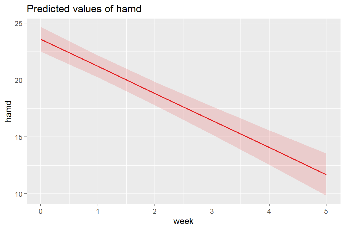
Adding the random slopes didn’t change the estimates for the fixed effects much.

12.5.4 Estimated Marginal Means and Emperical Bayes Plots

data_long %>% 
  dplyr::mutate(pred_fixed = predict(fit_lmer_week_RIAS_reml, 
                                     re.form = NA,               # fixed effects only
                                     newdata = .)) %>% 
  dplyr::mutate(pred_wrand = predict(fit_lmer_week_RIAS_reml,    # fixed and random effects together
                                     newdata = .)) %>%               
  ggplot(aes(x = week,
             y = hamd,
             group = id)) +
  geom_line(aes(y        = pred_wrand,
                color    = "BLUP",
                size     = "BLUP",
                linetype = "BLUP")) +
  geom_line(aes(y        = pred_fixed,
                color    = "Marginal",
                size     = "Marginal",
                linetype = "Marginal")) +
  theme_bw() +
  scale_color_manual(name   = "Type of Prediction",
                     values = c("BLUP"     = "gray50",
                                "Marginal" = "blue"))  +
  scale_size_manual(name    = "Type of Prediction",
                    values = c("BLUP"      = .5,
                               "Marginal" = 1.25))  +
  scale_linetype_manual(name   = "Type of Prediction",
                        values = c("BLUP"     = "longdash",
                                   "Marginal" = "solid"))  +
  theme(legend.position = c(0, 0),
        legend.justification = c(-0.1, -0.1),
        legend.background = element_rect(color = "black"),
        legend.key.width = unit(1.5, "cm")) +
  labs(x = "Weeks Since Baseline",
       y = "Estimated Hamilton Depression Score")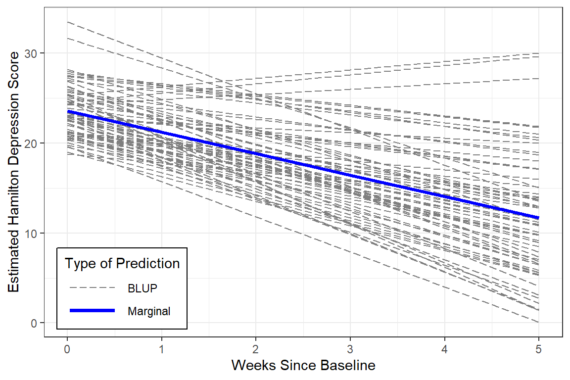

BLUPs are also refered to as Empirical Bayes Estimates and may be extracted from a model fit. In this cases there will be a specific intercept ((Intercept)) and time slope (week) for each individual or person (id).

12.5.4.1 Fixed Effects

Marginal Model = within-subject effects

fixef(fit_lmer_week_RIAS_reml)

(Intercept)        week 
  23.577044   -2.377047

12.5.4.2 Random Effects

between-subjects effects

ranef(fit_lmer_week_RIAS_reml)$id %>% 
  head()                                 # only the first 6 participants

    (Intercept)       week
101   1.0572022 -2.1151378
103   3.6707900 -0.4832479
104   2.6727551 -1.5008819
105  -3.0413391  0.2264496
106   0.3154240  1.0254750
107  -0.6148994 -0.4297385

12.5.4.3 BLUPs or Empirical Bayes Estimates

fixed effects + random effects

coef(fit_lmer_week_RIAS_reml)$id %>% 
  head()                                 # only the first 6 participants

    (Intercept)      week
101    24.63425 -4.492185
103    27.24783 -2.860295
104    26.24980 -3.877929
105    20.53571 -2.150598
106    23.89247 -1.351572
107    22.96214 -2.806786

We can create a scatterplot of these to see the correlation between them.

coef(fit_lmer_week_RIAS_reml)$id %>% 
  ggplot(aes(x = week,
             y = `(Intercept)`)) +
  geom_point() +
  geom_hline(yintercept = fixef(fit_lmer_week_RIAS_reml)["(Intercept)"],
             linetype = "dashed") +
  geom_vline(xintercept = fixef(fit_lmer_week_RIAS_reml)["week"],
             linetype = "dashed") +
  geom_smooth(method = "lm") +
  labs(title = "Hedeker's Figure 4.4 on page 59",
       subtitle = "Reisby data: Estimated random effects",
       x = "Week Change in Depression",
       y = "Baseline Depression Level") +
  theme_bw()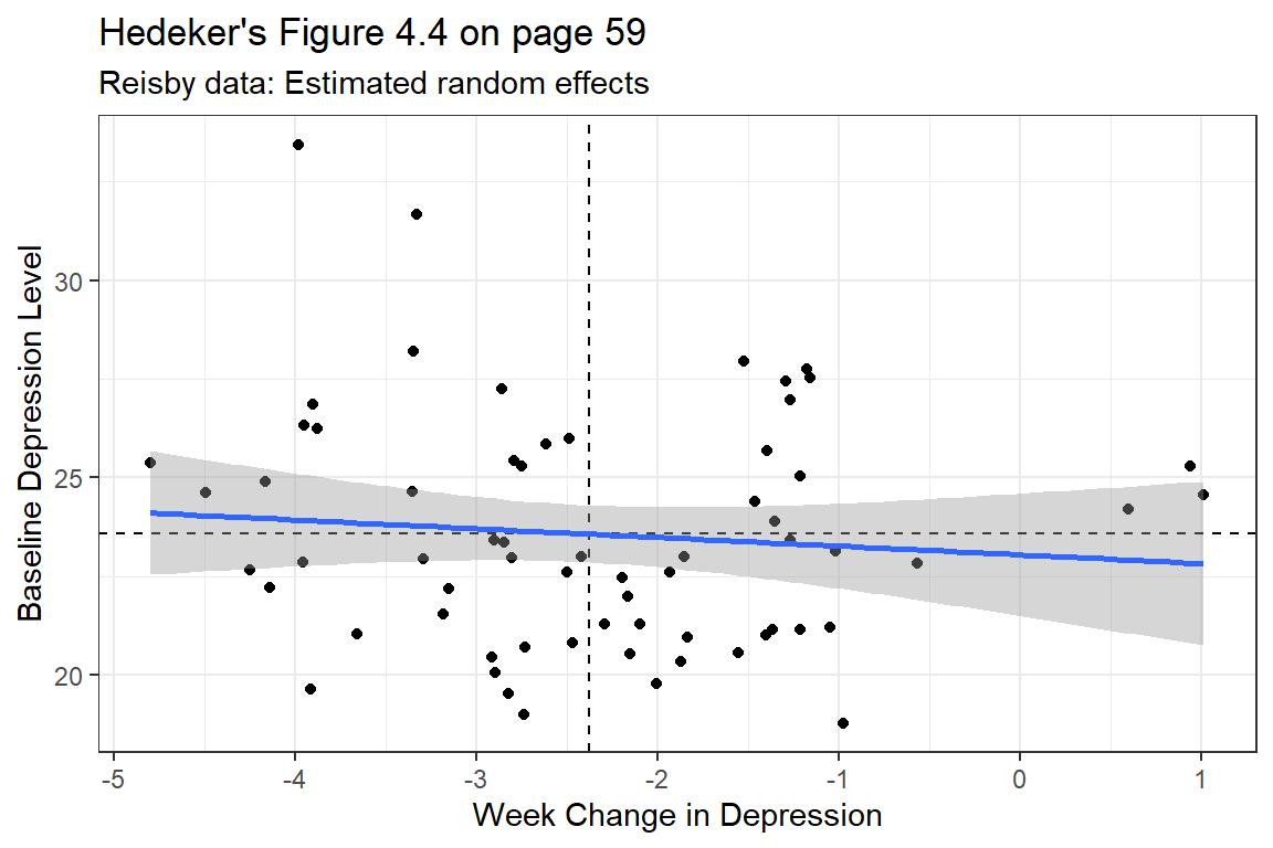

12.6 MLM: Coding of Time

So far we have used the variable week to denote time as weeks since baseline = week $\in 0, 1, 2, 3, 4, 5$.

But We could CENTER week at the middle of the study (week = 2.5).

12.6.1 Fit the Model

fit_lmer_week_RIAS_reml_wc <- 
  lmerTest::lmer(hamd ~ I(week-2.5) + (I(week-2.5)|id), #     MLM-RIAS
                 data = data_long,
                 REML = TRUE)

12.6.2 Table of Parameter Estimates

apaSupp::tab_lmers(list("Random Intercepts" = fit_lmer_week_RIAS_reml, 
                        " And Random Slopes" = fit_lmer_week_RIAS_reml_wc),
                   caption = "MLM: Null models fit w/REML",
                   general_note = "Hedeker table table 4.5 on page 58 and table 4.6 on page 61, except using REML here instead of ML")

**Table 12.9**
MLM: Null models fit w/REML
	Random Intercepts			And Random Slopes
Variable	b	(SE)	p	b	(SE)	p
(Intercept)	23.58	(0.55)	< .001***	17.63	(0.56)	< .001***
week	-2.38	(0.21)	< .001***
I(week - 2.5)				-2.38	(0.21)	< .001***
id.var__(Intercept)	12.94			18.85
id.cov__(Intercept).week	-1.48
id.var__week	2.13
Residual.var__Observation	12.21			12.21
id.cov__(Intercept).I(week - 2.5)				3.84
id.var__I(week - 2.5)				2.13
AIC	2,232			2,232
BIC	2,255			2,255
Log-likelihood	-1,110			-1,110
Note. Hedeker table table 4.5 on page 58 and table 4.6 on page 61, except using REML here instead of ML
* p < .05. p < .01. * p < .001.

Unchanged
model fit: AIC, BIC, -2LL, residual variance
fixed effect of week
variance for random intercepts
Changed
fixed intercept
variance for random slopes
covariance between random intercepts and random slopes
model fit: AIC, BIC, -2LL, residual variance
fixed effect of week
variance for random intercepts
Changed
fixed intercept
variance for random slopes
covariance between random intercepts and random slopes

12.6.3 Estimated Marginal Means and Emperical Bayes Plots

data_long %>% 
  dplyr::mutate(pred_fixed = predict(fit_lmer_week_RIAS_reml_wc, 
                                     re.form = NA, 
                                     newdata = .)) %>%               # fixed effects only
  dplyr::mutate(pred_wrand = predict(fit_lmer_week_RIAS_reml_wc, 
                                     newdata = .)) %>%               # fixed and random effects together
  ggplot(aes(x = week,
             y = hamd,
             group = id)) +
  geom_line(aes(y        = pred_wrand,
                color    = "BLUP",
                size     = "BLUP",
                linetype = "BLUP")) +
  geom_line(aes(y        = pred_fixed,
                color    = "Marginal",
                size     = "Marginal",
                linetype = "Marginal")) +
  theme_bw() +
  scale_color_manual(name   = "Type of Prediction",
                     values = c("BLUP"     = "gray50",
                                "Marginal" = "blue"))  +
  scale_size_manual(name    = "Type of Prediction",
                    values = c("BLUP"      = .5,
                               "Marginal" = 1.25))  +
  scale_linetype_manual(name   = "Type of Prediction",
                        values = c("BLUP"     = "longdash",
                                   "Marginal" = "solid"))  +
  theme(legend.position = c(0, 0),
        legend.justification = c(-0.1, -0.1),
        legend.background = element_rect(color = "black"),
        legend.key.width = unit(1.5, "cm")) +
  labs(x = "Weeks Since Baseline",
       y = "Estimated Hamilton Depression Score (HD)")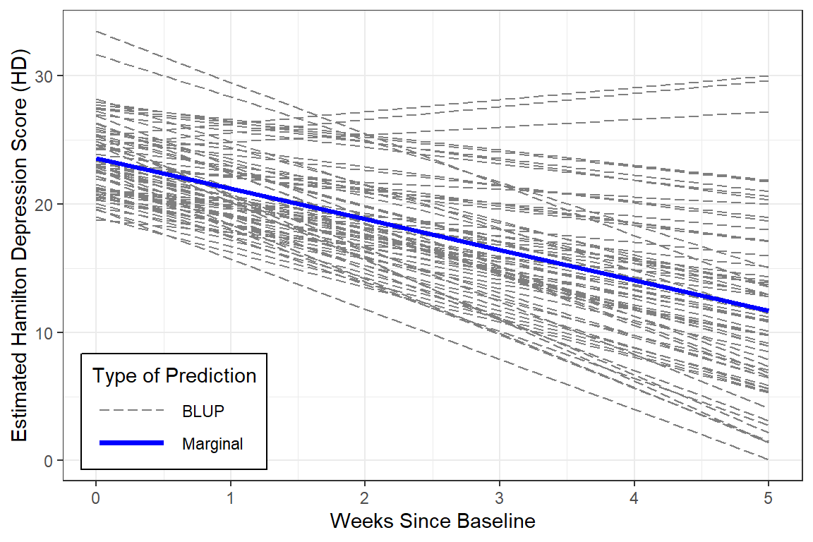

Again, centering time doesn’t change the interpretation at all, since there are no interactions.

12.7 MLM: Effect of DIagnosis on Time Trends (Fixed Interaction)

The researcher specifically wants to know if the trajectory over time differs for the two types of depression. This translates into a fixed effects interaction between time and group.

Start by comapring random intercepts only (RI) to a random intercetps and slopes (RIAS) model.

12.7.1 Fit the Models

fit_lmer_week_RIAS_ml <- lmerTest::lmer(hamd ~ week + (week|id), 
                                        data = data_long,
                                        REML = FALSE)

fit_lmer_wkdx_RIAS_ml <- lmerTest::lmer(hamd ~ week*endog + (week|id), 
                                        data = data_long,
                                        REML = FALSE)

12.7.2 Estimated Marginal Meanse Plot

interactions::interact_plot(fit_lmer_wkdx_RIAS_ml,
                            pred = week,
                            modx = endog,
                            legend.main = "Type of Depression",
                            interval = TRUE,
                            main.title = "Hedeker's Table 4.7 on page 64") +
  theme_bw() +
  labs(x = "Weeks Since Baseline",
       y = "Estimated Marginal Mean\nHamilton Depression Scores (HD)") +
  theme(legend.background = element_rect(color = "black"),
        legend.position = c(0, 0),
        legend.justification = c(-0.1, -0.1),
        legend.key.width = unit(1.75, "cm"))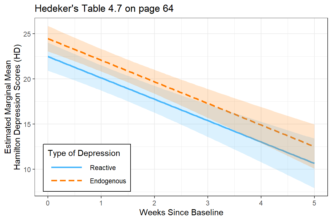

12.7.3 Likelihood Ratio Test

anova(fit_lmer_week_RIAS_ml, 
      fit_lmer_wkdx_RIAS_ml, 
      model.names = c("Just Time", 
                      "Time X Dx"))

Data: data_long
Models:
Just Time: hamd ~ week + (week | id)
Time X Dx: hamd ~ week * endog + (week | id)
          npar    AIC    BIC  logLik -2*log(L)  Chisq Df Pr(>Chisq)
Just Time    6 2231.0 2254.6 -1109.5    2219.0                     
Time X Dx    8 2230.9 2262.3 -1107.5    2214.9 4.1083  2     0.1282

apaSupp::tab_lmer_fits(list("Just Time" = fit_lmer_week_RIAS_ml, 
                            "Time X Dx" = fit_lmer_wkdx_RIAS_ml))

**Table 12.10**
Comparison of MLM Performane Metrics
Model	AIC	BIC	RMSE	$R^2$
Model	AIC	BIC	RMSE	Conditional	Marginal
Just Time	2231.04	2254.60	3.00	.767	.305
Time X Dx	2230.93	2262.34	3.00	.768	.324
Note. Larger $R^2$ values indicated better performance. Smaller values indicated better performance for Akaike's Information Criteria (AIC), Bayesian information criteria (BIC), and Root Mean Squared Error (RMSE).

The more complicated model (including the moderating effect of diagnosis) is NOT supported.

The more complicated model (including the moderating effect of diagnosis) is NOT supported.

12.8 MLM: Quadratic Trend

12.8.1 Fit the Model

fit_lmer_quad_RIAS_ml <- 
  lmerTest::lmer(hamd ~ week + I(week^2) + (week+ I(week^2)|id), 
                 data = data_long,
                 REML = FALSE,
                 control = lmerControl(optimizer = "optimx",    # get it to converge
                                       calc.derivs = FALSE,
                                       optCtrl = list(method = "nlminb",
                                                      starttests = FALSE,
                                                      kkt = FALSE)))

12.8.2 Table of Parameter Estimates

apaSupp::tab_lmers(list("Linear Trend" = fit_lmer_week_RIAS_ml,
                        "Quadratic Trend" = fit_lmer_quad_RIAS_ml),
                  caption = "MLM: RIAS models fit w/ML",
                  general_note = "Hedeker table 4.5 on page 58 and table 5.1 on page 84")

**Table 12.11**
MLM: RIAS models fit w/ML
	Linear Trend			Quadratic Trend
Variable	b	(SE)	p	b	(SE)	p
(Intercept)	23.58	(0.55)	< .001***	23.76	(0.55)	< .001***
week	-2.38	(0.21)	< .001***	-2.63	(0.48)	< .001***
I(week^2)				0.05	(0.09)	.562
id.var__(Intercept)	12.63			10.44
id.cov__(Intercept).week	-1.42			-0.92
id.var__week	2.08			6.64
Residual.var__Observation	12.22			10.52
id.cov__(Intercept).I(week^2)				-0.11
id.cov__week.I(week^2)				-0.94
id.var__I(week^2)				0.19
AIC	2,231			2,228
BIC	2,255			2,267
Log-likelihood	-1,110			-1,104
Note. Hedeker table 4.5 on page 58 and table 5.1 on page 84
* p < .05. p < .01. * p < .001.

12.8.3 Likelihood Ratio Test

anova(fit_lmer_week_RIAS_ml, fit_lmer_quad_RIAS_ml)

Data: data_long
Models:
fit_lmer_week_RIAS_ml: hamd ~ week + (week | id)
fit_lmer_quad_RIAS_ml: hamd ~ week + I(week^2) + (week + I(week^2) | id)
                      npar    AIC    BIC  logLik -2*log(L) Chisq Df Pr(>Chisq)
fit_lmer_week_RIAS_ml    6 2231.0 2254.6 -1109.5    2219.0                    
fit_lmer_quad_RIAS_ml   10 2227.7 2266.9 -1103.8    2207.7 11.39  4    0.02252
                       
fit_lmer_week_RIAS_ml  
fit_lmer_quad_RIAS_ml *
---
Signif. codes:  0 '***' 0.001 '**' 0.01 '*' 0.05 '.' 0.1 ' ' 1

apaSupp::tab_lmer_fits(list("Linear Trend" = fit_lmer_week_RIAS_ml,
                            "Quadratic Trend" = fit_lmer_quad_RIAS_ml))

**Table 12.12**
Comparison of MLM Performane Metrics
Model	AIC	BIC	RMSE	$R^2$
Model	AIC	BIC	RMSE	Conditional	Marginal
Linear Trend	2231.04	2254.60	3.00	.767	.305
Quadratic Trend	2227.65	2266.92	2.66	.799	.306
Note. Larger $R^2$ values indicated better performance. Smaller values indicated better performance for Akaike's Information Criteria (AIC), Bayesian information criteria (BIC), and Root Mean Squared Error (RMSE).

Even though the Wald test did not find the quadratic fixed time trend to be significant at the population level (marginal), the LRT and Bayes Factor both find that including the quadratic terms improves the model’s fit.

12.8.4 Estimated Marginal Means Plot

fixef(fit_lmer_quad_RIAS_ml)

(Intercept)        week   I(week^2) 
23.76024931 -2.63257550  0.05148118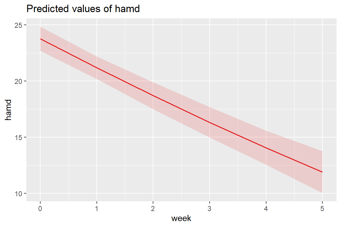

sjPlot::plot_model(fit_lmer_quad_RIAS_ml,
                   type = "pred",
                   terms = "week")

At the population level, the curviture is very slight.

12.8.5 BLUPs or Emperical Bayes Estimates

coef(fit_lmer_quad_RIAS_ml)$id

    (Intercept)        week    I(week^2)
101    25.16568 -5.28320574  0.150797898
103    27.50745 -3.43491942  0.119893070
104    25.99802 -3.09402774 -0.176874809
105    21.01143 -2.95260695  0.164661310
106    23.64346 -0.74434288 -0.141869439
107    22.70272 -1.98456635 -0.179102723
108    22.40954 -4.72427333  0.316018273
113    22.70934 -0.40481066 -0.023811547
114    21.71498 -4.51594039  0.305503426
115    21.54597 -2.55735173  0.139468215
117    20.68538 -3.87700598  0.196726431
118    25.37072 -2.57668561 -0.047612788
120    21.54365 -2.02855857  0.175311125
121    22.58018 -1.75376620 -0.038803501
123    19.25422 -2.87313328  0.017544440
302    21.58631 -3.89089208  0.294415462
303    22.46073 -3.40753346  0.044347424
304    24.67540 -0.37917905 -0.166163234
305    21.27401 -3.68029891 -0.010284082
308    23.09149 -2.47011784  0.005957118
309    22.90665 -1.55838475 -0.062497756
310    23.05813 -5.82989110  0.392498095
311    21.32624 -1.62725872  0.056409374
312    20.97726 -0.80436962 -0.285840159
313    21.61301 -4.45108736  0.355814846
315    25.23222 -4.58343575  0.080215319
316    27.75570 -1.45599106  0.069628465
318    20.56471 -0.29407613 -0.235305940
319    22.38191 -4.51711680  0.466348104
322    24.93396  1.26790220 -0.042514973
327    19.82906 -3.17596440  0.466785078
328    23.74557  1.29271519 -0.129016269
331    21.92610 -1.83150085 -0.074414325
333    23.11845 -0.64673576 -0.127985644
334    27.19413 -6.33064836  0.497609399
335    22.72436 -2.57422920  0.010288104
337    25.62004 -2.06605757 -0.118351519
338    22.89846 -0.54280685 -0.095535665
339    24.27805 -4.99289355  0.444970899
344    22.43029 -4.34889767  0.557803881
345    27.22530 -1.03850791 -0.044993297
346    24.66105 -2.09385824  0.138720526
347    20.11424 -3.85554369  0.239872680
348    23.42448 -4.05934237  0.152401519
349    20.49507 -3.30476908  0.269603183
350    23.29831 -3.86555309  0.351771472
351    27.85601 -2.54762022 -0.174399140
352    21.86126 -2.47215900  0.305550241
353    25.44900 -1.25790274 -0.261971309
354    26.94737  0.07804051 -0.289825508
355    24.47061 -2.72957880 -0.141018009
357    25.37351 -0.82942992 -0.114172123
360    24.04648  1.73526367 -0.131110574
361    25.48488 -7.37196846  0.953493451
501    27.83193 -1.46847456 -0.003542252
502    22.99362 -4.51402369  0.038610170
504    20.80203 -2.67923854  0.167676919
505    20.96545 -6.31342799  0.490342679
507    26.25982  0.08284338 -0.277546394
603    25.55711 -3.23920867  0.099754365
604    26.04324 -6.06910895  0.284967399
606    24.47425 -3.73161413 -0.178377690
607    31.08954  1.15555205 -1.091096102
608    23.46557 -4.87963004  0.180135655
609    25.91657 -2.23143282 -0.347100805
610    30.62473 -0.54534562 -0.593020846

For Illustration, two cases have been hand selected: id = 115 and 610.

fun_115 <- function(week){
  coef(fit_lmer_quad_RIAS_ml)$id["115", "(Intercept)"] +
    coef(fit_lmer_quad_RIAS_ml)$id["115", "week"] * week +
    coef(fit_lmer_quad_RIAS_ml)$id["115", "I(week^2)"] * week^2
}


fun_610 <- function(week){
  coef(fit_lmer_quad_RIAS_ml)$id["610", "(Intercept)"] +
    coef(fit_lmer_quad_RIAS_ml)$id["610", "week"] * week +
    coef(fit_lmer_quad_RIAS_ml)$id["610", "I(week^2)"] * week^2
}

data_long %>% 
  dplyr::mutate(pred_fixed = predict(fit_lmer_quad_RIAS_ml, 
                                     re.form = NA,
                                     newdata = .)) %>% # fixed effects only
  dplyr::mutate(pred_wrand = predict(fit_lmer_quad_RIAS_ml,
                                     newdata = .)) %>%               # fixed and random effects together
  ggplot(aes(x = week,
             y = hamd,
             group = id)) +
  stat_function(fun = fun_115) +          # add cure for ID = 115
  stat_function(fun = fun_610) +          # add cure for ID = 610
  geom_line(aes(y        = pred_fixed),
            color    = "blue",
            size     = 1.25)  +
  theme_bw() +
  theme(legend.position = c(0, 0),
        legend.justification = c(-0.1, -0.1),
        legend.background = element_rect(color = "black"),
        legend.key.width = unit(1.5, "cm")) +
  labs(x = "Weeks Since Baseline",
       y = "Estimated Hamilton Depression Scores (HD)",
       title = "Similar to Hedeker's Figure 5.3 on page 84",
       subtitle = "Marginal Mean show in thicker blue\nBLUPs for two of the participant in thinner black")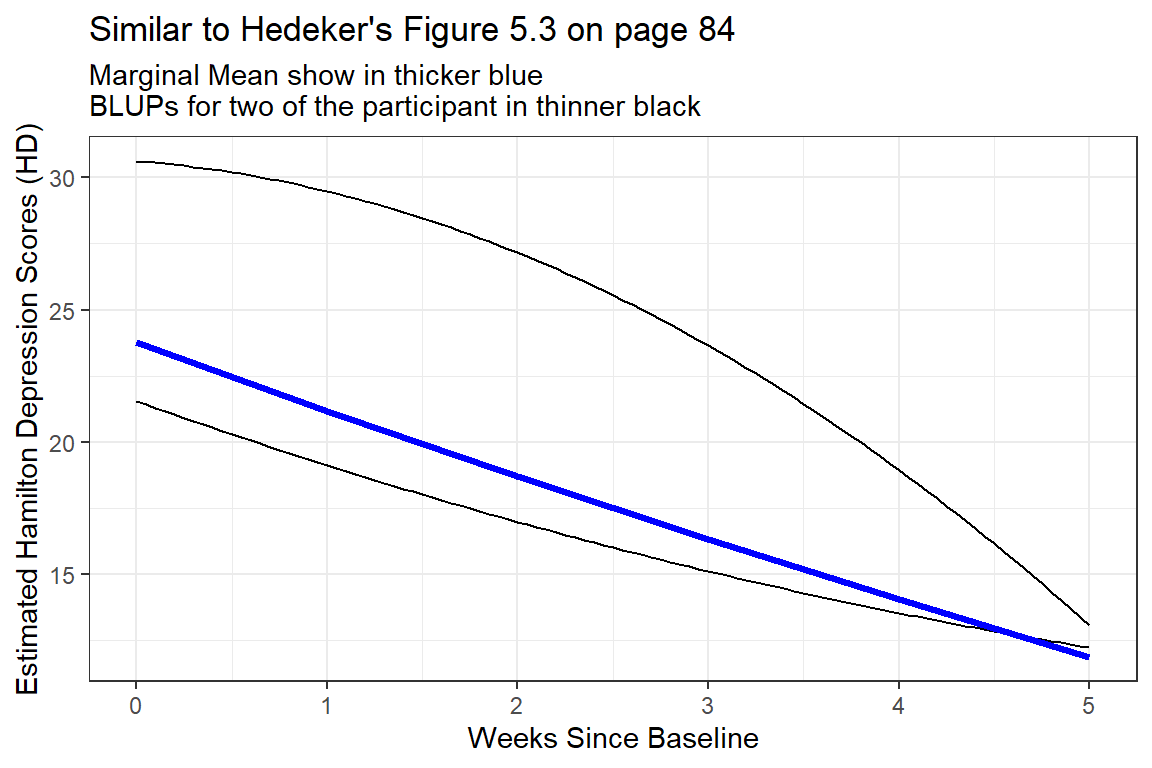

Figure 12.1
Two Example BLUPS for two different participants

These two individuals have quite different curvatures and illustrated how this type of curvatures in person-specific trajectories may end up cancelling each other out to arrive at a fairly linear marginal model.

12.8.6 Estimated Marginal Means and Emperical Bayes Plots

Note: although the BLUPs are shown for all participants, the predictions are just connects and are therefore slightly jagged and now smoother like the lines on the plot above.

data_long %>% 
  dplyr::mutate(pred_fixed = predict(fit_lmer_quad_RIAS_ml, 
                                     re.form = NA,
                                     newdata = .)) %>% # fixed effects only
  dplyr::mutate(pred_wrand = predict(fit_lmer_quad_RIAS_ml,
                                     newdata = .)) %>%               # fixed and random effects together
  ggplot(aes(x = week,
             y = hamd,
             group = id)) +
  geom_line(aes(y        = pred_wrand,
                color    = "BLUP",
                size     = "BLUP",
                linetype = "BLUP")) +
  geom_line(aes(y        = pred_fixed,
                color    = "Marginal",
                size     = "Marginal",
                linetype = "Marginal")) +
  theme_bw() +
  scale_color_manual(name   = "Type of Prediction",
                     values = c("BLUP"     = "gray50",
                                "Marginal" = "blue"))  +
  scale_size_manual(name    = "Type of Prediction",
                    values = c("BLUP"      = .5,
                               "Marginal" = 1.25))  +
  scale_linetype_manual(name   = "Type of Prediction",
                        values = c("BLUP"     = "longdash",
                                   "Marginal" = "solid"))  +
  theme(legend.position = c(0, 0),
        legend.justification = c(-0.1, -0.1),
        legend.background = element_rect(color = "black"),
        legend.key.width = unit(1.5, "cm")) +
  labs(x = "Weeks Since Baseline",
       y = "Estimated Hamilton Depression Scores",
       title = "Hedeker's Figure 5.4 on page 85")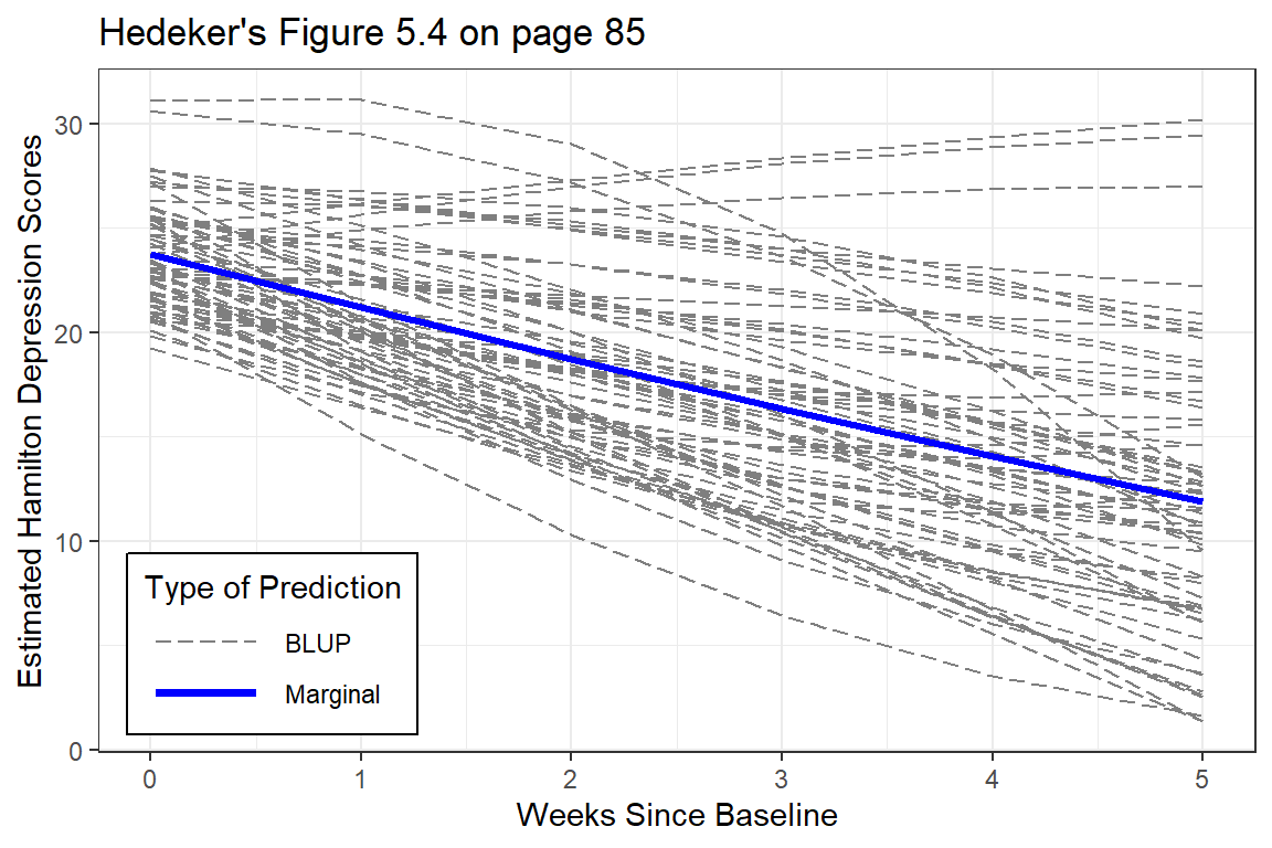

Figure 12.2
EStimated curvilinear trends

At the person-level, the curvature is very diverse (heterogeneous). Some individuals have accelerating downward tend while other have accelerating upward trends.

The improvement that the curvi-linear model provides in describing change across time is perhaps modest.