16 Ex: Logistic - Maternal Risk (Hoffman)

Maternal Risk Factor for Low Birth Weight Delivery

Compiled: October 15, 2025

16.1 PREPARATION

16.1.1 Load Packages

# install.packages("remotes")
# remotes::install_github("sarbearschwartz/apaSupp") # 9/17/2025

library(tidyverse)   
library(flextable)
library(apaSupp)       # not on CRAN, get from GitHub (above) 
library(naniar)
library(interactions)
library(effects)

16.1.2 Load Data

More complex example demonstrating modeling decisions

Another set of data from a study investigating predictors of low birth weight

• id infant’s unique identification number

Dependent variable (DV) or outcome

• low Low birth weight (outcome)

• 0 = birth weight >2500 g (normal)

• 1 = birth weight < 2500 g (low))

• bwt actual infant birth weight in grams (ignore for now)

Independent variables (IV) or predictors

• age Age of mother, in years
• lwt Mother’s weight at last menstrual period, in pounds
• ftv Number of physician visits in 1st trimester: 0 = None, 1 = One, … 6 = six
• race Race: 1 = White, 2 = Black, 3 = Other
• ptl History of premature labor: 0 = None, 1 = One, 2 = two, 3 = three
• ht History of hypertension: 1 = Yes, 0 = No
• smoke Smoking status during pregnancy:1 = Yes, 0 = No
• ui Uterine irritability: 1 = Yes, 0 = No

The data is saved in a text file (.txt) without any labels.

df_txt <- read.table("https://raw.githubusercontent.com/CEHS-research/data/master/Regression/lowbwt.txt", 
                     header = TRUE, 
                     sep = "", 
                     na.strings = "NA", 
                     dec = ".", 
                     strip.white = TRUE)

tibble::glimpse(df_txt)

Rows: 189
Columns: 11
$ id    <int> 85, 86, 87, 88, 89, 91, 92, 93, 94, 95, 96, 97, 98, 99, 100, 101…
$ low   <int> 0, 0, 0, 0, 0, 0, 0, 0, 0, 0, 0, 0, 0, 0, 0, 0, 0, 0, 0, 0, 0, 0…
$ age   <int> 19, 33, 20, 21, 18, 21, 22, 17, 29, 26, 19, 19, 22, 30, 18, 18, …
$ lwt   <int> 182, 155, 105, 108, 107, 124, 118, 103, 123, 113, 95, 150, 95, 1…
$ race  <int> 2, 3, 1, 1, 1, 3, 1, 3, 1, 1, 3, 3, 3, 3, 1, 1, 2, 1, 3, 1, 3, 1…
$ smoke <int> 0, 0, 1, 1, 1, 0, 0, 0, 1, 1, 0, 0, 0, 0, 1, 1, 0, 1, 0, 1, 0, 0…
$ ptl   <int> 0, 0, 0, 0, 0, 0, 0, 0, 0, 0, 0, 0, 0, 1, 0, 0, 0, 0, 0, 0, 0, 0…
$ ht    <int> 0, 0, 0, 0, 0, 0, 0, 0, 0, 0, 0, 0, 1, 0, 0, 0, 0, 0, 0, 0, 0, 0…
$ ui    <int> 1, 0, 0, 1, 1, 0, 0, 0, 0, 0, 0, 0, 0, 1, 0, 0, 0, 0, 1, 0, 0, 1…
$ ftv   <int> 0, 3, 1, 2, 0, 0, 1, 1, 1, 0, 0, 1, 0, 2, 0, 0, 0, 3, 0, 1, 2, 3…
$ bwt   <int> 2523, 2551, 2557, 2594, 2600, 2622, 2637, 2637, 2663, 2665, 2722…

16.1.3 Wrangle Data

df_mom <- df_txt %>% 
  dplyr::mutate(id = factor(id)) %>% 
  dplyr::mutate(low = low %>% 
                  factor() %>% 
                  forcats::fct_recode("birth weight >2500 g (normal)" = "0",
                                      "birth weight < 2500 g (low)"   = "1")) %>% 
  dplyr::mutate(race = race %>% 
                  factor() %>% 
                  forcats::fct_recode("White" = "1",
                                      "Black" = "2",
                                      "Other" = "3")) %>% 
  dplyr::mutate(ptl_any = as.numeric(ptl > 0)) %>%         # collapse into 0 = none vs. 1 = at least one
  dplyr::mutate(ptl = factor(ptl)) %>%                     # declare the number of pre-term labors to be a factor: 0, 1, 2, 3
  dplyr::mutate_at(vars(smoke, ht, ui, ptl_any),           # declare all there variables to be factors with the same two levels
                   factor,
                   levels = 0:1,
                   labels = c("No", "Yes")) 

Display the structure of the ‘clean’ version of the dataset

str(df_mom)

'data.frame':   189 obs. of  12 variables:
 $ id     : Factor w/ 189 levels "4","10","11",..: 60 61 62 63 64 65 66 67 68 69 ...
 $ low    : Factor w/ 2 levels "birth weight >2500 g (normal)",..: 1 1 1 1 1 1 1 1 1 1 ...
 $ age    : int  19 33 20 21 18 21 22 17 29 26 ...
 $ lwt    : int  182 155 105 108 107 124 118 103 123 113 ...
 $ race   : Factor w/ 3 levels "White","Black",..: 2 3 1 1 1 3 1 3 1 1 ...
 $ smoke  : Factor w/ 2 levels "No","Yes": 1 1 2 2 2 1 1 1 2 2 ...
 $ ptl    : Factor w/ 4 levels "0","1","2","3": 1 1 1 1 1 1 1 1 1 1 ...
 $ ht     : Factor w/ 2 levels "No","Yes": 1 1 1 1 1 1 1 1 1 1 ...
 $ ui     : Factor w/ 2 levels "No","Yes": 2 1 1 2 2 1 1 1 1 1 ...
 $ ftv    : int  0 3 1 2 0 0 1 1 1 0 ...
 $ bwt    : int  2523 2551 2557 2594 2600 2622 2637 2637 2663 2665 ...
 $ ptl_any: Factor w/ 2 levels "No","Yes": 1 1 1 1 1 1 1 1 1 1 ...

tibble::glimpse(df_mom)

Rows: 189
Columns: 12
$ id      <fct> 85, 86, 87, 88, 89, 91, 92, 93, 94, 95, 96, 97, 98, 99, 100, 1…
$ low     <fct> birth weight >2500 g (normal), birth weight >2500 g (normal), …
$ age     <int> 19, 33, 20, 21, 18, 21, 22, 17, 29, 26, 19, 19, 22, 30, 18, 18…
$ lwt     <int> 182, 155, 105, 108, 107, 124, 118, 103, 123, 113, 95, 150, 95,…
$ race    <fct> Black, Other, White, White, White, Other, White, Other, White,…
$ smoke   <fct> No, No, Yes, Yes, Yes, No, No, No, Yes, Yes, No, No, No, No, Y…
$ ptl     <fct> 0, 0, 0, 0, 0, 0, 0, 0, 0, 0, 0, 0, 0, 1, 0, 0, 0, 0, 0, 0, 0,…
$ ht      <fct> No, No, No, No, No, No, No, No, No, No, No, No, Yes, No, No, N…
$ ui      <fct> Yes, No, No, Yes, Yes, No, No, No, No, No, No, No, No, Yes, No…
$ ftv     <int> 0, 3, 1, 2, 0, 0, 1, 1, 1, 0, 0, 1, 0, 2, 0, 0, 0, 3, 0, 1, 2,…
$ bwt     <int> 2523, 2551, 2557, 2594, 2600, 2622, 2637, 2637, 2663, 2665, 27…
$ ptl_any <fct> No, No, No, No, No, No, No, No, No, No, No, No, No, Yes, No, N…

16.2 EXPLORATORY DATA ANALYSIS

16.2.1 Missing Data

df_mom %>% 
  dplyr::select("Race" = race, 
                "Low Birth Weight Delivery" = low,
                "Age, years" = age, 
                "Weight, pounds" = lwt, 
                "1st Tri Dr Visits" = ftv, 
                "History of Premature Labor, any" = ptl_any, 
                "History of Premature Labor, number" = ptl, 
                "Smoking During pregnancy" = smoke, 
                "History of Hypertension" = ht, 
                "Uterince Irritability" = ui) %>% 
  naniar::miss_var_summary() %>%
  dplyr::select(Variable = variable,
                n = n_miss) %>% 
  flextable::flextable() %>% 
  apaSupp::theme_apa(caption = "Missing Data by Variable")

Table 16.1
Missing Data by Variable

Variable	n
Race	0
Low Birth Weight Delivery	0
Age, years	0
Weight, pounds	0
1st Tri Dr Visits	0
History of Premature Labor, any	0
History of Premature Labor, number	0
Smoking During pregnancy	0
History of Hypertension	0
Uterince Irritability	0

16.2.2 Summary

df_mom %>% 
  dplyr::select("Low Birth Weight Delivery" = low,
                "Race" = race, 
                "Age, yrs" = age, 
                "Weight, lbs" = lwt, 
                "1st Tri Dr Visits" = ftv, 
                "Hx of Premature Labor, number" = ptl, 
                "Hx Premature Labor, any" = ptl_any, 
                "Hx of Hypertension" = ht, 
                "Smoking During pregnancy" = smoke, 
                "Uterince Irritability" = ui) %>% 
  apaSupp::tab_freq(caption = "Summary of Categorical Variables")

Table 16.2
Summary of Categorical Variables

		Statistic (N=189)
Low Birth Weight Delivery
birth weight >2500 g (normal)		130 (68.8%)
birth weight < 2500 g (low)		59 (31.2%)
Race
White		96 (50.8%)
Black		26 (13.8%)
Other		67 (35.4%)
Hx of Premature Labor, number
0		159 (84.1%)
1		24 (12.7%)
2		5 (2.6%)
3		1 (0.5%)
Hx Premature Labor, any
No		159 (84.1%)
Yes		30 (15.9%)
Hx of Hypertension
No		177 (93.7%)
Yes		12 (6.3%)
Smoking During pregnancy
No		115 (60.8%)
Yes		74 (39.2%)
Uterince Irritability
No		161 (85.2%)
Yes		28 (14.8%)

df_mom %>% 
  dplyr::select("Low Birth Weight Delivery" = low,
                "Race" = race,  
                "Age, yrs" = age, 
                "Weight, lbs" = lwt, 
                "1st Tri Dr Visits" = ftv,
                "Hx Premature Labor, any" = ptl_any, 
                "Hx Premature Labor, number" = ptl, 
                "Hx Hypertension" = ht, 
                "Smoking During pregnancy" = smoke, 
                "Uterince Irritability" = ui) %>% 
  apaSupp::tab_desc(caption = "Summary of Continuous Variables")

Table 16.3
Summary of Continuous Variables

	NA	M	SD	min	Q1	Mdn	Q3	max
Age, yrs	0	23.24	5.30	14	19.00	23	26.00	45
Weight, lbs	0	129.81	30.58	80	110.00	121	140.00	250
1st Tri Dr Visits	0	0.79	1.06	0	0.00	0	1.00	6
Note. N = 189. NA = not available or missing; Mdn = median; Q1 = 25th percentile; Q3 = 75th percentile.

16.3 UNADJUSTED

Unadjusted Models

16.3.1 Fit Models

fit_glm_race  <- glm(low ~ race,    family = binomial(link = "logit"), data = df_mom)
fit_glm_age   <- glm(low ~ age,     family = binomial(link = "logit"), data = df_mom)
fit_glm_lwt   <- glm(low ~ lwt,     family = binomial(link = "logit"), data = df_mom)
fit_glm_ftv   <- glm(low ~ ftv,     family = binomial(link = "logit"), data = df_mom)

fit_glm_ptl   <- glm(low ~ ptl_any, family = binomial(link = "logit"), data = df_mom)
fit_glm_ht    <- glm(low ~ ht,      family = binomial(link = "logit"), data = df_mom)
fit_glm_smoke <- glm(low ~ smoke,   family = binomial(link = "logit"), data = df_mom)
fit_glm_ui    <- glm(low ~ ui,      family = binomial(link = "logit"), data = df_mom)

16.3.2 Parameter Tables

Note: the parameter estimates here are for the LOGIT scale, not the odds ration (OR) or even the probability.

apaSupp::tab_glms(list(fit_glm_race, fit_glm_age, fit_glm_lwt, fit_glm_ftv),
                  narrow = TRUE,
                  fit = NA,
                  pr2 = "tjur")

Table 16.4
Compare Generalized Regression Models

	Model 1		Model 2		Model 3		Model 4
Variable	OR	95% CI	OR	95% CI	OR	95% CI	OR	95% CI
race
White	—	—
Black	2.33	[0.93, 5.77]
Other	1.89	[0.96, 3.76]
age			0.95	[0.89, 1.01]
lwt					0.99	[0.97, 1.00]*
ftv							0.87	[0.63, 1.17]
pseudo-R²	.026		.014		.031		.004
Note. N = 189. CI = confidence interval.Coefficient of determination estiamted by Tjur's psuedo R-squared
* p < .05. ** p < .01. *** p < .001.

apaSupp::tab_glms(list(fit_glm_ptl, fit_glm_ht, fit_glm_smoke, fit_glm_ui),
                  narrow = TRUE,
                  fit = NA,
                  pr2 = "tjur")

Table 16.5
Compare Generalized Regression Models

	Model 1		Model 2		Model 3		Model 4
Variable	OR	95% CI	OR	95% CI	OR	95% CI	OR	95% CI
ptl_any
No	—	—
Yes	4.32	[1.94, 9.95]***
ht
No			—	—
Yes			3.37	[1.03, 11.83]*
smoke
No					—	—
Yes					2.02	[1.08, 3.80]*
ui
No							—	—
Yes							2.58	[1.13, 5.88]*
pseudo-R²	.073		.023		.026		.029
Note. N = 189. CI = confidence interval.Coefficient of determination estiamted by Tjur's psuedo R-squared
* p < .05. ** p < .01. *** p < .001.

16.4 MAIN EFFECTS ONLY

Main-effects multiple logistic regression model

fit_glm_mains <- glm(low ~ race + age + lwt + ftv + ptl_any + ht + smoke + ui,
                     family = binomial(link = "logit"), 
                     data = df_mom)

apaSupp::tab_glm(fit_glm_mains,
                 var_labels = c(race = "Race",
                                age = "Age, yrs",
                                lwt = "Prior Weight, lbs",
                                ftv = "First Tri Visits",
                                ptl_any = "Hx Premature Labor",
                                ht = "Hx Hypertension",
                                smoke = "Smoking",
                                ui = "Uterine Irritability"),
                 show_single_row = c("ptl_any", "smoke", "ht", "ui"),
                 vif = FALSE) %>% 
  flextable::width(j = 1, width = 1.75)

Table 16.6
Parameter Estimates for Generalized Linear Regression

	Odds Ratio			Logit Scale
Variable	OR	95% CI		b	(SE)		Wald	LRT
Race								.039*
White	—	—		—	—
Black	3.38	[1.19, 9.81]		1.219	(0.53)		.022*
Other	2.27	[0.95, 5.60]		.819	(0.45)		.069
Age, yrs	0.96	[0.89, 1.03]		-0.04	(0.04)		.302	.297
Prior Weight, lbs	0.99	[0.97, 1.00]		-0.02	(0.01)		.032*	.024*
First Tri Visits	1.05	[0.74, 1.48]		0.05	(0.18)		.772	.772
Hx Premature Labor	3.38	[1.38, 8.57]		1.22	(0.46)		.008**	.008**
Hx Hypertension	6.43	[1.66, 28.19]		1.86	(0.71)		.009**	.007**
Smoking	2.36	[1.07, 5.38]		0.86	(0.41)		.036*	.034*
Uterine Irritability	2.05	[0.82, 5.10]		0.72	(0.46)		.121	.124
(Intercept)				0.64	(1.22)		.598
pseudo-R²	.191
Note. N = 189. CI = confidence interval. Significance denotes Wald t-tests for individual parameter estimates, as well as Likelihood Ratio Tests (LRT) for single-predictor deletion. Coefficient of determination displays Tjur's pseudo-R².
* p < .05. ** p < .01. *** p < .001.

16.5 INTERACTIONS

Before removing non-significant main effects, test plausible interactions

Try the following interactions:

• Age and Weight

• Age and Smoking

• Weight and Smoking

fit_glm_mains_aw <- glm(low ~ race + age + lwt + ftv + ptl_any + ht + smoke + ui + age:lwt,
                        family = binomial(link = "logit"), 
                        data = df_mom)

fit_glm_mains_as <- glm(low ~ race + age + lwt + ftv + ptl_any + ht + smoke + ui + age:smoke,
                        family = binomial(link = "logit"), 
                        data = df_mom)

fit_glm_mains_ws <- glm(low ~ race + age + lwt + ftv + ptl_any + ht + smoke + ui + lwt:smoke,
                        family = binomial(link = "logit"), 
                        data = df_mom)

apaSupp::tab_glms(list("Age-Weight"     = fit_glm_mains_aw,
                       "Age-Smoking"    = fit_glm_mains_as,
                       "Weight-Smoking" = fit_glm_mains_ws),
                  var_labels = c(race = "Race",
                                 age = "Age, yrs",
                                 lwt = "Prior Weight, lbs",
                                 ftv = "First Tri Visits",
                                 ptl_any = "Hx Premature Labor",
                                 smoke = "Smoking",
                                 ht = "Hypertension",
                                 ui = "Uterine Irritability"),
                  narrow = TRUE,
                  show_single_row = c("ptl_any", "smoke", "ht", "ui"))

Table 16.7
Compare Generalized Regression Models

	Age-Weight		Age-Smoking		Weight-Smoking
Variable	OR	95% CI	OR	95% CI	OR	95% CI
Race
White	—	—	—	—	—	—
Black	3.36	[1.18, 9.78]*	3.10	[1.07, 9.18]*	3.44	[1.21, 9.99]*
Other	2.25	[0.94, 5.60]	2.18	[0.90, 5.41]	2.06	[0.85, 5.13]
Age, yrs	0.94	[0.67, 1.33]	0.93	[0.83, 1.03]	0.96	[0.89, 1.04]
Prior Weight, lbs	0.98	[0.92, 1.04]	0.99	[0.97, 1.00]*	0.98	[0.95, 1.00]*
First Tri Visits	1.05	[0.74, 1.48]	1.04	[0.73, 1.46]	1.03	[0.72, 1.44]
Hx Premature Labor	3.40	[1.38, 8.64]**	3.30	[1.35, 8.34]**	3.54	[1.44, 9.01]**
Hypertension	6.43	[1.66, 28.23]**	6.54	[1.69, 28.82]**	5.79	[1.48, 25.60]*
Smoking	2.35	[1.06, 5.36]*	0.57	[0.02, 18.96]	0.33	[0.01, 10.04]
Uterine Irritability	2.06	[0.82, 5.13]	2.20	[0.86, 5.59]	2.23	[0.88, 5.64]
age * lwt	1.00	[1.00, 1.00]
age * smoke
age * Yes			1.06	[0.92, 1.24]
lwt * smoke
lwt * Yes					1.02	[0.99, 1.04]
Fit Metrics
AIC	218.7		218.1		217.4
BIC	254.4		253.7		253.1
pseudo-R²
Tjur	.191		.192		.196
McFadden	.162		.164		.167
Note. N = 189. CI = confidence interval.Coefficient of determination estiamted with both Tjur and McFadden's psuedo R-squared
* p < .05. ** p < .01. *** p < .001.

apaSupp::tab_glm_fits(list("Only Mains"     = fit_glm_mains,
                           "Age-Weight"     = fit_glm_mains_aw,
                           "Age-Smoking"    = fit_glm_mains_as,
                           "Weight-Smoking" = fit_glm_mains_ws))

Table 16.8
Comparison of Generalized Linear Model Performane Metrics

			pseudo- $R^2$
Model	N	k	McFadden	Tjur	AIC	BIC	RMSE
Only Mains	189	10	.162	.191	216.75	249.17	0.42
Age-Weight	189	11	.162	.191	218.73	254.39	0.42
Age-Smoking	189	11	.164	.192	218.08	253.74	0.42
Weight-Smoking	189	11	.167	.196	217.42	253.08	0.42
Note. k = number of parameters estimated in each model. Larger $R^2$ values indicated better performance. Smaller values indicated better performance for Akaike's Information Criteria (AIC), Bayesian information criteria (BIC), and Root Mean Squared Error (RMSE).

anova(fit_glm_mains, fit_glm_mains_aw, test = 'LRT')

# A tibble: 2 × 5
  `Resid. Df` `Resid. Dev`    Df Deviance `Pr(>Chi)`
        <dbl>        <dbl> <dbl>    <dbl>      <dbl>
1         179         197.    NA  NA          NA    
2         178         197.     1   0.0190      0.890

anova(fit_glm_mains, fit_glm_mains_as, test = 'LRT')

# A tibble: 2 × 5
  `Resid. Df` `Resid. Dev`    Df Deviance `Pr(>Chi)`
        <dbl>        <dbl> <dbl>    <dbl>      <dbl>
1         179         197.    NA   NA         NA    
2         178         196.     1    0.669      0.413

anova(fit_glm_mains, fit_glm_mains_ws, test = 'LRT')

# A tibble: 2 × 5
  `Resid. Df` `Resid. Dev`    Df Deviance `Pr(>Chi)`
        <dbl>        <dbl> <dbl>    <dbl>      <dbl>
1         179         197.    NA    NA        NA    
2         178         195.     1     1.33      0.249

16.6 PARSAMONY

No interactions are significant Remove non-significant main effects

Since the mother’s age is theoretically a meaningful variable, it should probably be retained.

Remove “UI” since its not significant

fit_glm_trim <- glm(low ~  race + age + lwt + ptl_any + ht + smoke ,
                    family = binomial(link = "logit"), 
                    data = df_mom)

apaSupp::tab_glm(fit_glm_trim,
                 var_labels = c(race = "Race",
                                age = "Age, yrs",
                                lwt = "Prior Weight, lbs",
                                ptl_any = "Hx Premature Labor",
                                ht = "Hx Hypertension",
                                smoke = "Smoking"),
                 show_single_row = c("ptl_any", "smoke", "ht"),
                 lrt = FALSE,
                 vif = FALSE) %>% 
  flextable::width(j = 1, width = 1.75)

Table 16.9
Parameter Estimates for Generalized Linear Regression

	Odds Ratio			Logit Scale
Variable	OR	95% CI		b	(SE)		p
Race
White	—	—		—	—
Black	3.22	[1.13, 9.31]		1.168	(0.53)		.028*
Other	2.26	[0.96, 5.50]		.815	(0.44)		.066
Age, yrs	0.96	[0.89, 1.03]		-0.04	(0.04)		.255
Prior Weight, lbs	0.98	[0.97, 1.00]		-0.02	(0.01)		.028*
Hx Premature Labor	3.80	[1.57, 9.53]		1.33	(0.46)		.004**
Hx Hypertension	5.70	[1.49, 24.76]		1.74	(0.70)		.013*
Smoking	2.36	[1.08, 5.32]		0.86	(0.40)		.034*
(Intercept)				0.92	(1.20)		.442
pseudo-R²	.180
Note. N = 189. CI = confidence interval. Significance denotes Wald t-tests for parameter estimates. Coefficient of determination displays Tjur's pseudo-R².
* p < .05. ** p < .01. *** p < .001.

16.7 CENTER & SCALE

Since the mother’s age is theoretically a meaningful variable, it should probably be retained.

Revise so that age is interpreted in 5-year and pre-pregnancy weight in 20 lb increments and the intercept has meaning.

fit_glm_final <- glm(low ~ race + I((age - 20)/5) + I((lwt - 125)/20) 
                     + ptl_any + ht + smoke ,
                     family = binomial(link = "logit"), 
                     data = df_mom)

apaSupp::tab_glm(fit_glm_final,
                 var_labels = c("I((age - 20)/5)" = "Age, 5 yr",
                                "I((lwt - 125)/20)" = "Pre-Preg Weight, 20 lb",
                                race = "Race",
                                smoke = "Smoker",
                                ptl_any = "Prior Preterm Labor",
                                ht = "Hx Hypertension"),
                 p_note = "apa13",
                 show_single_row = c("smoke", "ptl_any", "ht"),
                 general_note = "Centering for age (20 yr) and weight (125 lbs)")

Table 16.10
Parameter Estimates for Generalized Linear Regression

	Odds Ratio			Logit Scale
Variable	OR	95% CI		b	(SE)		Wald	LRT	VIF
Race								.044*	1.49
White	—	—		—	—
Black	3.22	[1.13, 9.31]		1.168	(0.53)		.028*
Other	2.26	[0.96, 5.50]		.815	(0.44)		.066
Age, 5 yr	0.81	[0.55, 1.16]		-0.21	(0.19)		.255	.249	1.09
Pre-Preg Weight, 20 lb	0.73	[0.55, 0.95]		-0.31	(0.14)		.028*	.020*	1.29
Prior Preterm Labor	3.80	[1.57, 9.53]		1.33	(0.46)		.004**	.003**	1.08
Hx Hypertension	5.70	[1.49, 24.76]		1.74	(0.70)		.013*	.011*	1.15
Smoker	2.36	[1.08, 5.32]		0.86	(0.40)		.034*	.032*	1.35
(Intercept)				-1.86	(0.41)		< .001***
pseudo-R²	.180
Note. N = 189. CI = confidence interval; VIF = variance inflation factor. Significance denotes Wald t-tests for individual parameter estimates, as well as Likelihood Ratio Tests (LRT) for single-predictor deletion. Coefficient of determination displays Tjur's pseudo-R². Centering for age (20 yr) and weight (125 lbs)
* p < .05. *** p < .001.

16.8 Probe & Plot

16.8.1 focus: Compare Races with prior weight and hypertension

interactions::interact_plot(model = fit_glm_final,

                            pred = lwt,
                            modx = race,
                            legend.main = "Race",
                            mod2 = ht,
                            mod2.labels = c("History of Hypertension: No",
                                            "History of Hypertension: Yes"))  +
  theme_bw() +
  theme(legend.position = "inside",
        legend.position.inside = c(.5, 1),
        legend.justification = c(1.1, 1.1),
        legend.background = element_rect(color = "black"),
        legend.key.width = unit(1.5, "cm")) +
  scale_y_continuous(labels = scales::percent_format()) +
  labs(x = "Mother's Weight Pre-Pregnancy, pounds",
       y = "Predicted Probability\nBaby has Low Birth Weight (< 2500 grams)",
       linetype = "Race") +
  scale_linetype_manual(values = c("solid", "longdash", "dotted"))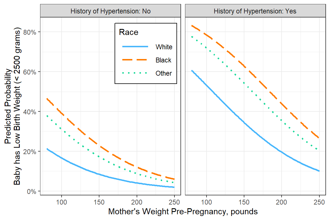

effects::Effect(mod = fit_glm_trim,
                focal.predictors = c("lwt", "race", "ptl_any", "ht", "smoke"),
                xlevels = list(lwt = seq(from = 80, to = 250, by = 5))) %>% 
  data.frame() %>%
  dplyr::filter(race != "Other") %>% 
  dplyr::mutate(risk = interaction(ptl_any, ht, smoke) %>% 
                  factor() %>% 
                  forcats::fct_recode("(0) None"               = "No.No.No",
                                      "(1) Preterm"            = "Yes.No.No" ,
                                      "(1) Ht"                 = "No.Yes.No" ,
                                      "(1) Smoking"            = "No.No.Yes" ,
                                      "(2) Preterm & Ht"       = "Yes.Yes.No" ,
                                      "(2) Ht & Smoking"       = "No.Yes.Yes" ,
                                      "(2) Preterm & Smoking"  = "Yes.No.Yes",
                                      "(3) All Three"          = "Yes.Yes.Yes") %>% 
                  forcats::fct_reorder(fit) %>% 
                  forcats::fct_rev()) %>%  

  ggplot(aes(x = lwt,
             y = fit)) +
  geom_line(aes(color = risk,
                linetype = risk,
                linewidth = risk)) +
  theme_bw() +
  facet_grid(~ race) +
  scale_linetype_manual(values = c("solid", 
                                   "longdash", "dotdash", "dashed", 
                                   "solid", "solid", "solid", 
                                   "solid")) +
  scale_linewidth_manual(values = c(1.5, 
                                    1.25, 1.25, 1.25, 
                                    .75, .75, .75, 
                                    .5)) +
  scale_color_manual(values = c("black", 
                                "red", "coral", "orange", 
                                "purple", "dodgerblue", "cyan3",  
                                "green4")) +
  scale_y_continuous(labels = scales::percent_format()) +
  labs(x = "Mother's Weight Pre-Pregnancy, pounds",
       y = "Predicted Probability\nBaby has Low Birth Weight (< 2500 grams)",
       color    = "Risk Factors:",
       linetype = "Risk Factors:",
       linewidth= "Risk Factors:") +
  theme(#legend.position = "bottom",
        legend.key.width = unit(1.5, "cm"))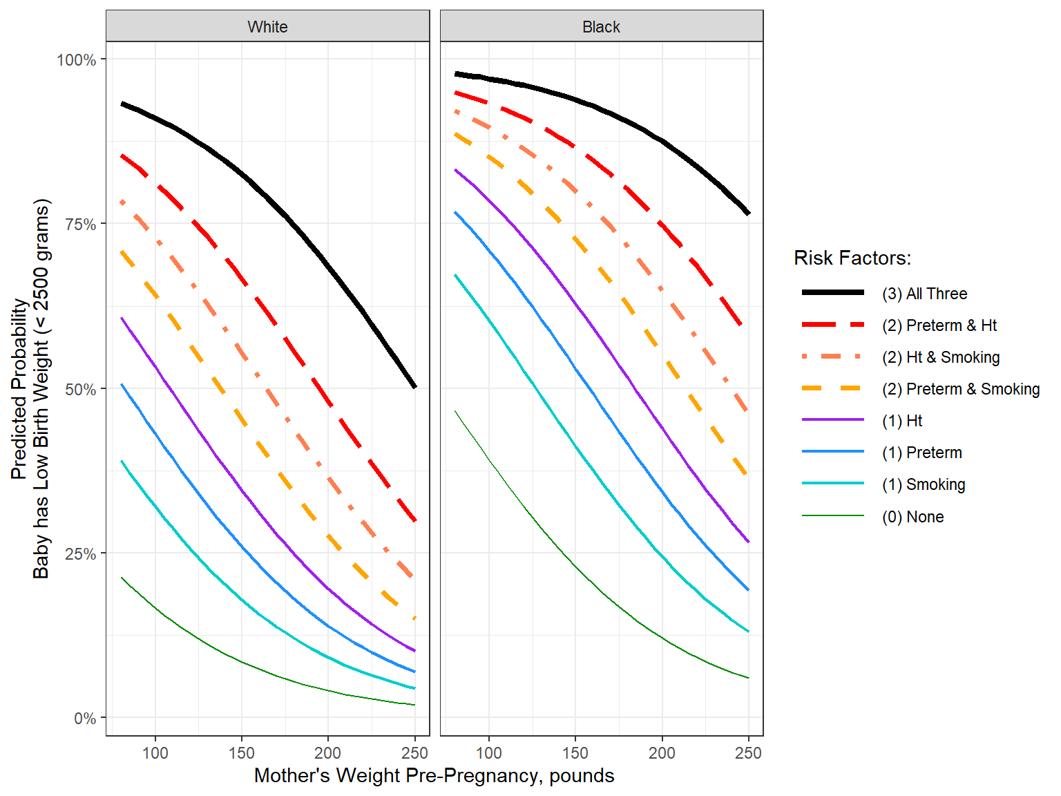 

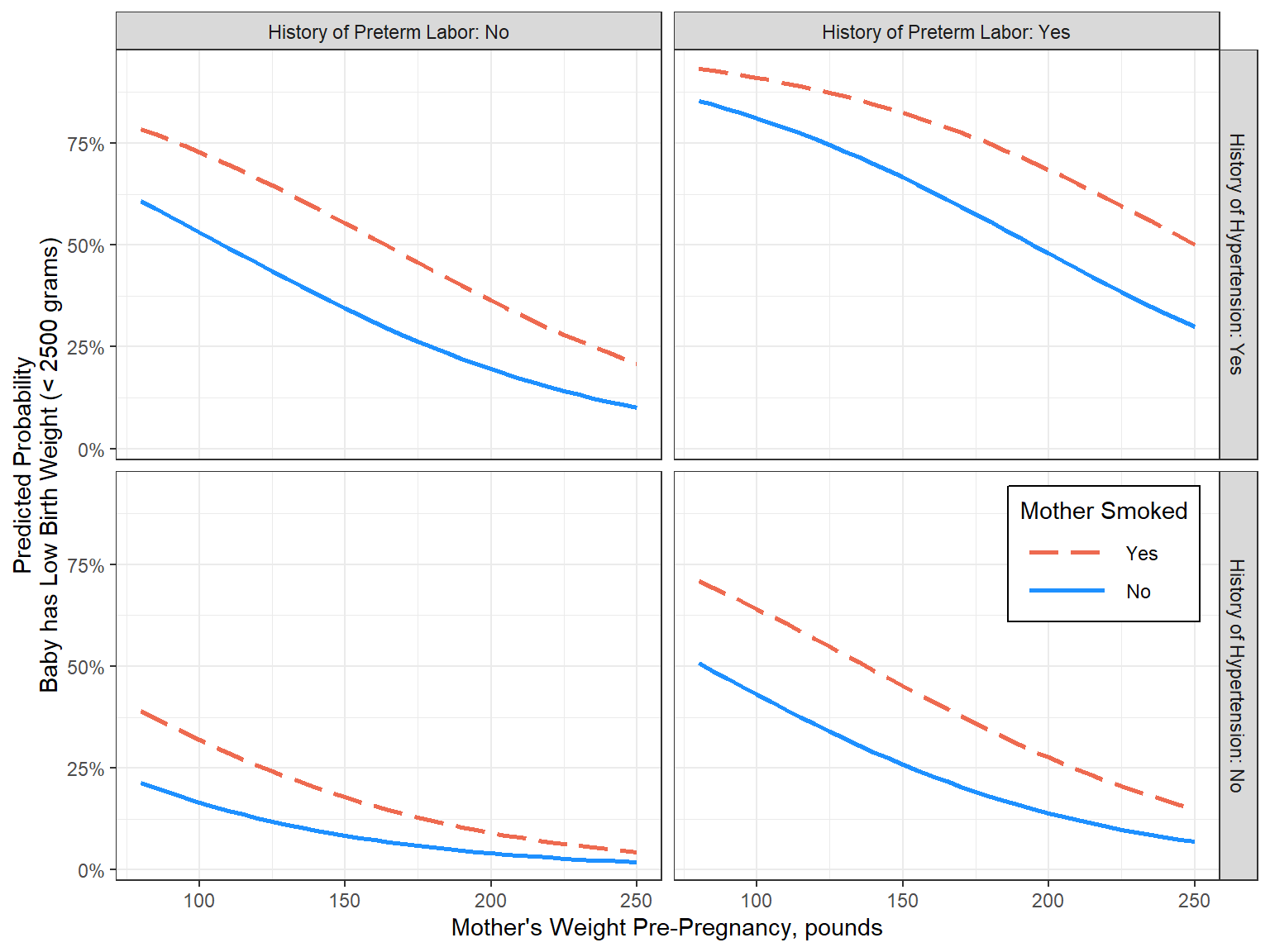
16.8.1.1 Focus on: Mother’s weight and smoking status during pregnancy, as well as history of any per-term labor and hypertension

Illustates risk given the mother is 20 years old and white

effects::Effect(mod = fit_glm_final,
                focal.predictors = c("race", "lwt", "smoke", "ptl_any", "ht"),
                fixed.predictors = list(age = 20),

                xlevels = list(lwt = seq(from = 80, to = 250, by = 5))) %>% 
  data.frame() %>% 
  dplyr::filter(race == "White") %>% 
  dplyr::mutate(smoke = forcats::fct_rev(smoke)) %>% 
  dplyr::mutate(ptl_any_labels = glue::glue("History of Preterm Labor: {ptl_any}")) %>% 
  dplyr::mutate(ht_labels = glue::glue("History of Hypertension: {ht}") %>% forcats::fct_rev()) %>% 
  ggplot(aes(x = lwt,
             y = fit)) +
  geom_line(aes(color = smoke,
                linetype = smoke),
            linewidth = 1) +
  theme_bw() +
  facet_grid(ht_labels ~ ptl_any_labels) +
  scale_y_continuous(labels = scales::percent_format()) +
  labs(x = "Mother's Weight Pre-Pregnancy, pounds",
       y = "Predicted Probability\nBaby has Low Birth Weight (< 2500 grams)",
       color    = "Mother Smoked",
       linetype = "Mother Smoked") +
  theme(legend.position = "inside",
        legend.position.inside = c(1, .5),
        legend.justification = c(1.1, 1.15),
        legend.background = element_rect(color = "black"),
        legend.key.width = unit(1.5, "cm")) +
  scale_linetype_manual(values = c("longdash", "solid")) +
  scale_color_manual(values = c( "coral2", "dodger blue"))