2 D&H Ch 2 - Simple Regression: “Minigolf”

Darlington & Hayes, Chapter 2

# install.packages("remotes")
# remotes::install_github("sarbearschwartz/apaSupp")
# remotes::install_github("ddsjoberg/gtsummary")

library(magrittr)       
library(tidyverse)   
library(broom)     
library(naniar)
library(corrplot)   
library(GGally)
library(gtsummary)
library(apaSupp)
library(performance)
library(interactions)
library(effects)
library(emmeans)
library(car)
library(ggResidpanel)
library(modelsummary)
library(ppcor)
library(jtools)
library(olsrr)
library(DescTools)
library(effectsize)
library(ggpubr)

2.1 PURPOSE

2.1.1 Research Question

Examine the relationship between the number of points won when playing mini golf and the number of times a player has played mini golf before.

2.1.2 Data Description

Manually enter the data set provided on page 18 in Table 2.1

df_golf <- data.frame(ID = 1:23,
                      X = c(0, 0, 
                            1, 1, 1, 
                            2, 2, 2, 2, 
                            3, 3, 3, 3, 3, 
                            4, 4, 4, 4,
                            5, 5, 5, 
                            6, 6),
                      Y = c(2, 3, 
                            2, 3, 4,
                            2, 3, 4, 5,
                            2, 3, 4, 5, 6,
                               3, 4, 5, 6,
                                  4, 5, 6,
                                     5, 6)) %>% 
  dplyr::mutate(ID = as.character(ID)) %>% 
  dplyr::mutate(across(c(X, Y), as.integer))  

tibble::glimpse(df_golf)

Rows: 23
Columns: 3
$ ID <chr> "1", "2", "3", "4", "5", "6", "7", "8", "9", "10", "11", "12", "13"…
$ X  <int> 0, 0, 1, 1, 1, 2, 2, 2, 2, 3, 3, 3, 3, 3, 4, 4, 4, 4, 5, 5, 5, 6, 6
$ Y  <int> 2, 3, 2, 3, 4, 2, 3, 4, 5, 2, 3, 4, 5, 6, 3, 4, 5, 6, 4, 5, 6, 5, 6

2.2 VISUALIZATION

2.2.1 Full Table

This is Table 2.1 on page 18.

tab_df_golf <- df_golf %>% 
  dplyr::select(ID,
                "X\n'Previous Plays'" = X,
                "Y\n'Points Won'" = Y) %>% 
  flextable::flextable() %>% 
  apaSupp::theme_apa(caption = "D&H Table 2.1: Golfing Scores and Prior Plays") %>% 
  flextable::colformat_double(digits = 0)

This is how you save a table to Word.

flextable::save_as_docx(tab_df_golf,
                        path = "tables/tab_df_golf.docx")

tab_df_golf

``` ```{=html}

(\#tab:unnamed-chunk-49)D&H Table 2.1: Golfing Scores and Prior Plays

ID	X 'Previous Plays'	Y 'Points Won'
1	0	2
2	0	3
3	1	2
4	1	3
5	1	4
6	2	2
7	2	3
8	2	4
9	2	5
10	3	2
11	3	3
12	3	4
13	3	5
14	3	6
15	4	3
16	4	4
17	4	5
18	4	6
19	5	4
20	5	5
21	5	6
22	6	5
23	6	6

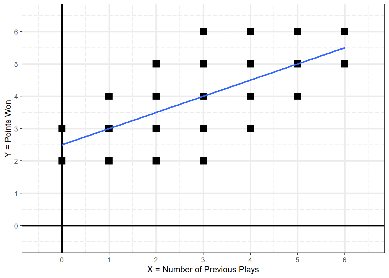
2.2.2 Scatterplot

This is Figure 2.1 on page 19

fig_blank <- df_golf %>% 
  ggplot(aes(x = X,
             y = Y)) +
  geom_vline(xintercept = 0,
             linewidth = 1) +
  geom_hline(yintercept = 0,
             linewidth = 1) +
  scale_x_continuous(breaks = 0:6, limits = c(-.5, 6.5)) +
  scale_y_continuous(breaks = 0:6, limits = c(-.5, 6.5)) +
  labs(x = "X = Number of Previous Plays",
       y = "Y = Points Won") +
  theme_bw() +
  theme(panel.grid.minor = element_line(linewidth = .5, 
                                        linetype = "longdash"),
        panel.grid.major = element_line(linewidth = 1))

fig_golf_scatter <- fig_blank +
  geom_point(shape = 15,
             size = 4) +
  geom_smooth(method = "lm",
              formula = y ~ x,
              se = FALSE) 

fig_golf_scatter 

Figure 2.1
D&H Figure 2.1 (page 19) A Simple Scatter Plot

This is how you save a plot, in three different formats.

ggsave(plot = fig_golf_scatter,
       file = "figures/fig_golf_scatter.png",
       width = 6,
       height = 4,
       units = "in")

ggsave(plot = fig_golf_scatter,
       file = "figures/fig_golf_scatter.jpg",
       width = 6,
       height = 4,
       units = "in")

ggsave(plot = fig_golf_scatter,
       file = "figures/fig_golf_scatter.tif",
       width = 6,
       height = 4,
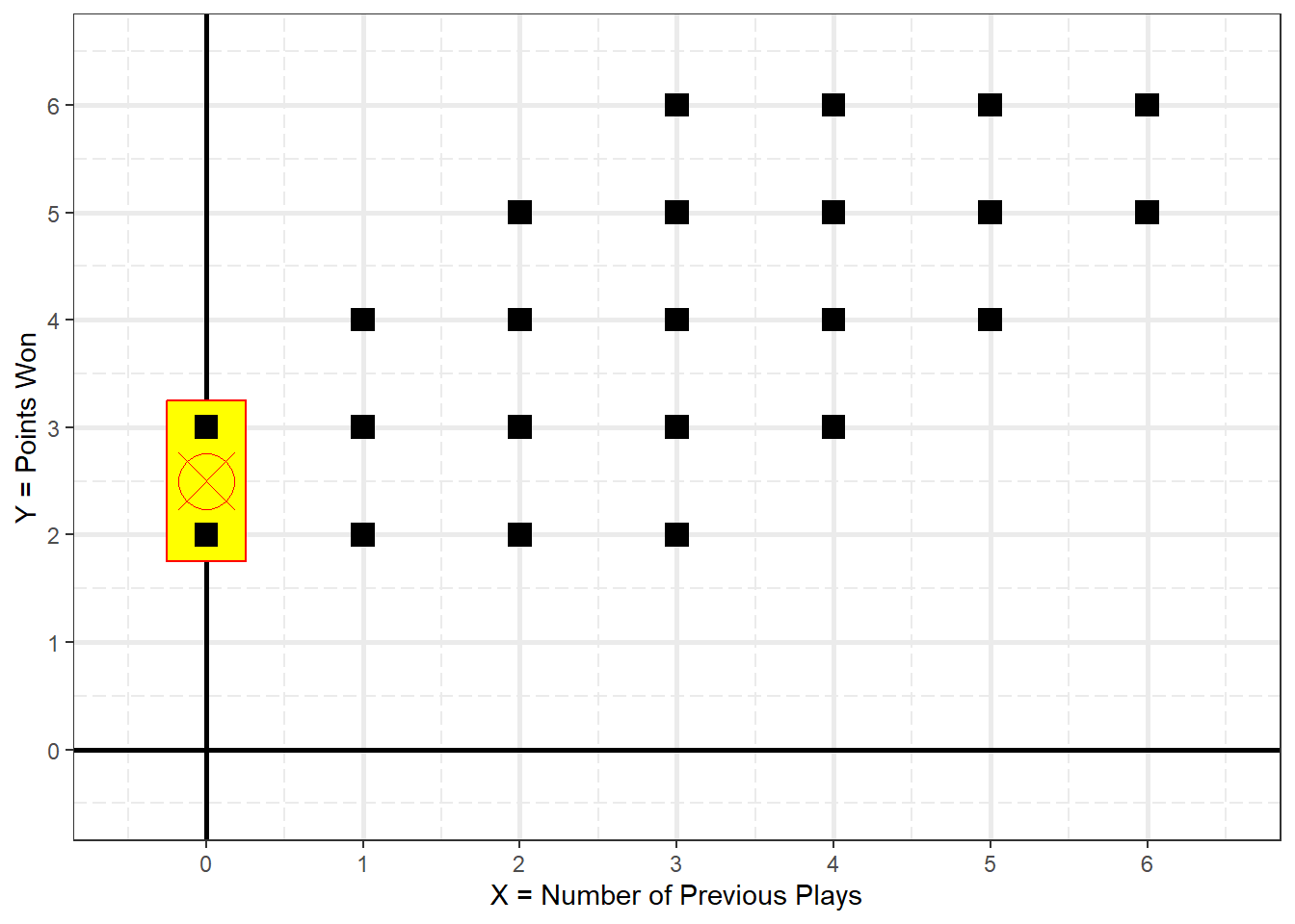
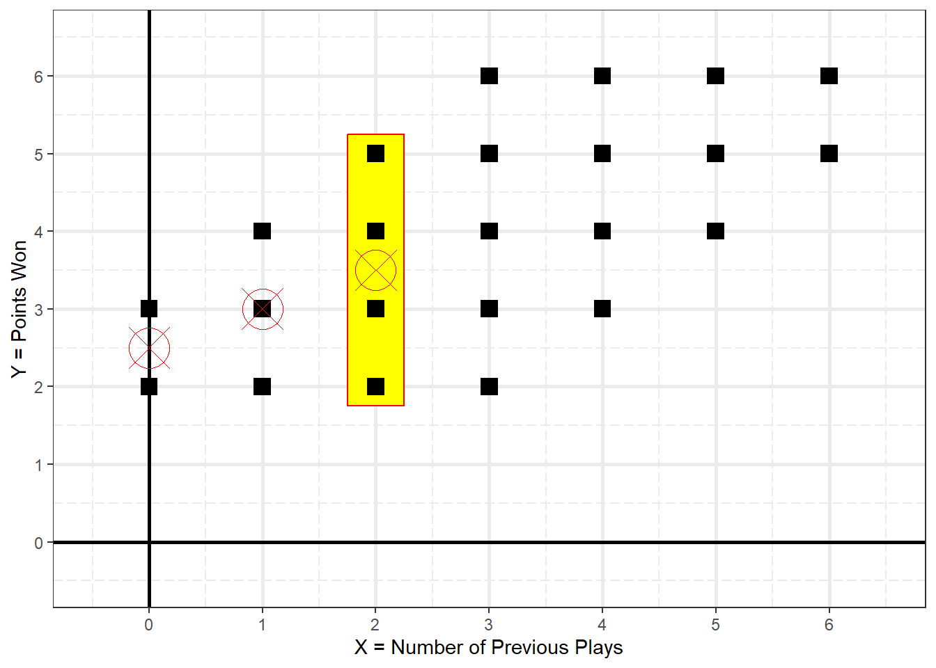
       units = "in")

2.2.3 Conditional Means

df_golf_means <- df_golf %>% 
  dplyr::group_by(X) %>% 
  dplyr::summarise(N = n(),
                   Y_bar = mean(Y)) %>% 
  dplyr::ungroup()

fig_blank +
  geom_rect(xmin = 0 - .25, xmax = 0 + 0.25,
            ymin = 2 - .25, ymax = 3 + 0.25,
            color = "red",
            alpha = .5,
            fill = "yellow") +
  geom_point(shape = 15,
             size = 4) +
  geom_point(data = df_golf_means %>% 
               dplyr::filter(X <= 0),
             aes(x = X,
                 y = Y_bar),
             color = "red",
             shape = 13,
             size = 10) 

Figure 2.2
Conditional Mean of Y When X = 0

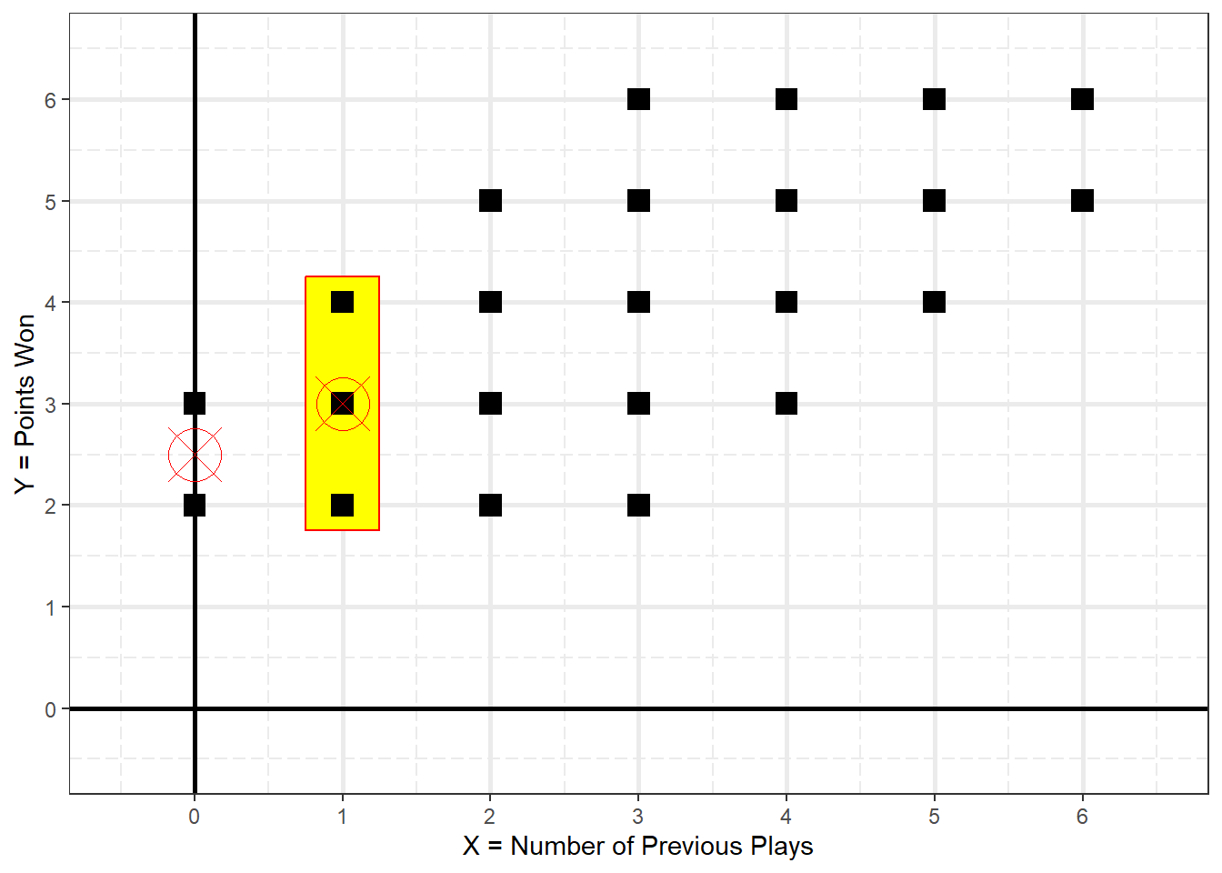
fig_blank +
  geom_rect(xmin = 1 - .25, xmax = 1 + 0.25,
            ymin = 2 - .25, ymax = 4 + 0.25,
            color = "red",
            alpha = .5,
            fill = "yellow") +
  geom_point(shape = 15,
             size = 4) +
  geom_point(data = df_golf_means %>% 
               dplyr::filter(X <= 1),
             aes(x = X,
                 y = Y_bar),
             color = "red",
             shape = 13,
             size = 10)

Figure 2.3
Conditional Mean of Y When X = 1

fig_blank +
  geom_rect(xmin = 2 - .25, xmax = 2 + 0.25,
            ymin = 2 - .25, ymax = 5 + 0.25,
            color = "red",
            alpha = .5,
            fill = "yellow") +
  geom_point(shape = 15,
             size = 4) +
  geom_point(data = df_golf_means %>% 
               dplyr::filter(X <= 2),
             aes(x = X,
                 y = Y_bar),
             color = "red",
             shape = 13,
             size = 10)

Figure 2.4
Conditional Mean of Y When X = 2

df_golf_means %>% 
  dplyr::select("X\nPrevious\nPlays" = N,
                "N\nNumber of\nObservations" = N,
                "Mean(Y)\nConditional Mean of\nPoints Won" = Y_bar) %>% 
  flextable::flextable() %>% 
  apaSupp::theme_apa(caption = "Golfing Scores and Prior Plays")  %>% 
  flextable::align(part = "body", align = "center") %>% 
  flextable::align(part = "head", align = "center")

``` ```{=html}

(\#tab:unnamed-chunk-60)Golfing Scores and Prior Plays

X Previous Plays	N Number of Observations	Mean(Y) Conditional Mean of Points Won
2	2	2.50
3	3	3.00
4	4	3.50
5	5	4.00
4	4	4.50
3	3	5.00
2	2	5.50

fig_golf_scatter +
  geom_point(data = df_golf_means,
             aes(x = X,
                 y = Y_bar),
             color = "red",
             shape = 13,
             size = 10)

Figure 2.5
Textbook’s Figure 2.2 (page 20) A Line Through Conditional Means

fig_blank +
  geom_point(shape = 15,
             size = 4,
             alpha = .3) +
  geom_smooth(method = "lm",
              formula = y ~ x,
              se = FALSE) +
  geom_point(x = 0,
             y = 2.5,
             color = "red",
             shape = 13,
             size = 10) +
  geom_segment(x = -.75, xend = -.1,
               y = 2.5, yend = 2.5,
               arrow = arrow(type = "closed"),
               color ="red") +
  geom_segment(x = 1, xend = 1,
               y = 3, yend = 4,
               arrow = arrow(length = unit(.3, "cm"),
                             type = "closed"),
               linewidth = 1,
               color = "darkgreen") +
  geom_segment(x = 1, xend = 3,
               y = 4, yend = 4,
               arrow = arrow(length = unit(.3, "cm"),
                             type = "closed"),
               linewidth = 1,
               color = "darkgreen") +
  annotate(x = 0.75, y = 3.5, 
           geom = "text", 
           label = "Rise 1",
           color = "darkgreen")+
  annotate(x = 2, y = 4.5, 
           geom = "text", 
           label = "Run 2",
           color = "darkgreen") +
  ggpubr::stat_regline_equation(label.x = 4.5,
                                label.y = 1,
                                size = 6)

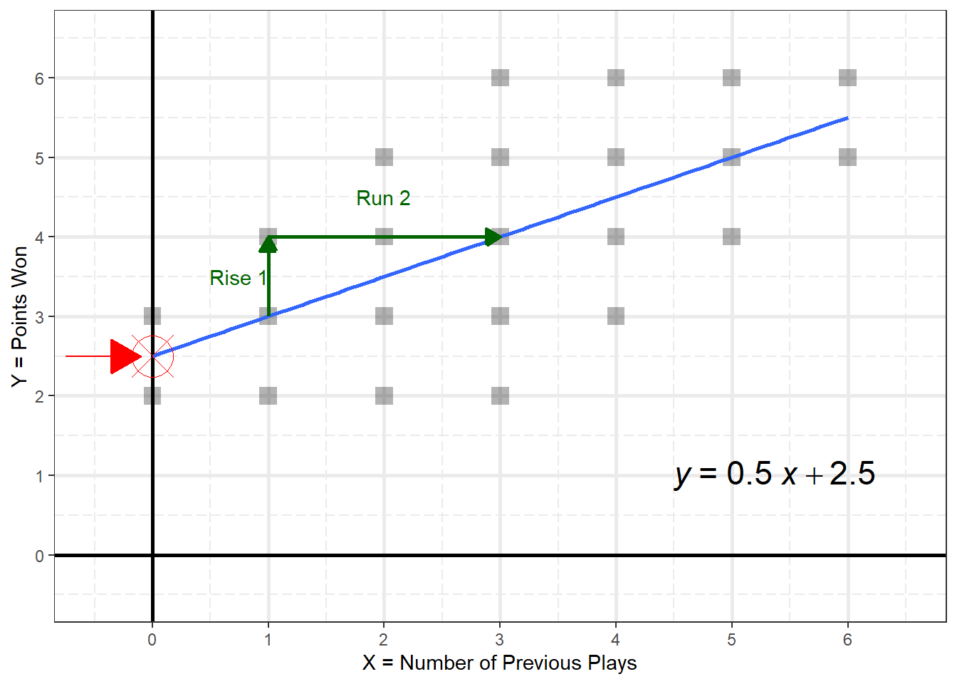
Figure 2.6
Y-Intercept and Slope of the Line

2.2.4 Y-intercept

Where the line crosses the vertical or y-axis

\[ b_0 = 2.5 \]

2.2.5 Slope

The incline or decline of the line

\[ b_1 = \frac{rise}{run} = \frac{1}{2} = 0.5 \]

2.2.6 Format

Standard slope-intercept form

\[ Y = mX + b \\ \text{or} \\ Y = b + mX \tag{Slope-Intercept Form} \]

In statistics:

\[ Y = b_0 + b_1X \tag{D&H 2.10} \]

So for this example, \(\hat{Y}\) is said “Y hat”.

\[ \hat{Y} = 2.5 + 0.5X \\ \text{or} \\ \widehat{\text{points}} = 2.58 + 0.5(\text{plays}) \]

2.3 HAND CALCULATIONS

ORDINARY LEAST SQUARES (OLS)

2.3.1 Estimates

The equation may be used to estimate predicted values (\(\hat{Y}\)) for each participant (\(i\)).

\[ \tag{OLS EQ} \widehat{Y_i} = 2.5 + 0.5X_i \]

The first participant (id = 1) had no previous plays (\(X = 0\)) and won two points (\(Y=2\))…

df_golf %>% 
  dplyr::filter(ID == "1")

# A tibble: 1 × 3
  ID        X     Y
  <chr> <int> <int>
1 1         0     2

…so we plug in the value of 0 for the variable \(x\) in the OLS Equation…

\[ \hat{Y} = 2.5 + 0.5 (0) \\ = 2.5 + 0 \\ = 2.5 \\ \]

…which gives a predicted value of two and a half points won (\(\hat{Y} = 2.5\)).

2.3.2 Residuals

The words error and residual mean the same thing (\(e\)).

\[ \tag{residuals} residual = \text{observed} - \text{predicted} \\ \text{or} \\ e_i= Y_i - \widehat{Y_i} \] For the first participant (ID = 1), this would be…

\[ e_1 = (2 - 2.5) = - 0.5 \]

This is because this participant won two points, which is a half a point LESS THAN the OLS equation which predicted two and a half points.

We can use this process to find the predicted values (\(\hat{Y}\)) and residuals (\(e\)) for all the participants in this sample (N = 23).

mean(df_golf$X)

[1] 3

mean(df_golf$Y)

[1] 4

df_golf_est <- df_golf %>% 
  dplyr::mutate(X2 = X^2) %>% 
  dplyr::mutate(Y2 = Y^2) %>% 
  dplyr::mutate(devX = X - 3) %>% 
  dplyr::mutate(devY = Y - 4) %>% 
  dplyr::mutate(devX_devY = devX*devY) %>% 
  dplyr::mutate(devX2 = devX^2) %>% 
  dplyr::mutate(devY2 = devY^2) %>%
  dplyr::mutate(estY = 2.5 + 0.5*X) %>%  # predicted
  dplyr::mutate(e = Y - estY) %>%        # deviation or residual
  dplyr::mutate(e2 = e^2)

df_golf_est_sums <- df_golf_est %>% 
  dplyr::summarise(across(where(is.numeric),~sum(.x))) %>% 
  dplyr::mutate(ID = "Sum") %>% 
  dplyr::select(ID, everything())

df_golf_est_means <- df_golf_est %>% 
  dplyr::summarise(across(where(is.numeric),~mean(.x))) %>% 
  dplyr::mutate(ID = "Mean") %>% 
  dplyr::select(ID, everything())

tab_golf_est <- df_golf_est %>% 
  dplyr::bind_rows(df_golf_est_sums) %>% 
  dplyr::bind_rows(df_golf_est_means) %>% 
  dplyr::select(ID, X, Y,estY, e, e2) %>% 
  flextable::flextable() %>% 
  apaSupp::theme_apa(caption = "D&H Tabel 2.2: Estimates and Residuals") %>% 
  flextable::hline(i = 23) 

tab_golf_est

``` ```{=html}

(\#tab:unnamed-chunk-69)D&H Tabel 2.2: Estimates and Residuals

ID	X	Y	estY	e	e2
1	0.00	2.00	2.50	-0.50	0.25
2	0.00	3.00	2.50	0.50	0.25
3	1.00	2.00	3.00	-1.00	1.00
4	1.00	3.00	3.00	0.00	0.00
5	1.00	4.00	3.00	1.00	1.00
6	2.00	2.00	3.50	-1.50	2.25
7	2.00	3.00	3.50	-0.50	0.25
8	2.00	4.00	3.50	0.50	0.25
9	2.00	5.00	3.50	1.50	2.25
10	3.00	2.00	4.00	-2.00	4.00
11	3.00	3.00	4.00	-1.00	1.00
12	3.00	4.00	4.00	0.00	0.00
13	3.00	5.00	4.00	1.00	1.00
14	3.00	6.00	4.00	2.00	4.00
15	4.00	3.00	4.50	-1.50	2.25
16	4.00	4.00	4.50	-0.50	0.25
17	4.00	5.00	4.50	0.50	0.25
18	4.00	6.00	4.50	1.50	2.25
19	5.00	4.00	5.00	-1.00	1.00
20	5.00	5.00	5.00	0.00	0.00
21	5.00	6.00	5.00	1.00	1.00
22	6.00	5.00	5.50	-0.50	0.25
23	6.00	6.00	5.50	0.50	0.25
Sum	69.00	92.00	92.00	0.00	25.00
Mean	3.00	4.00	4.00	0.00	1.09

2.3.3 Errors of Estimate

“Sum of the Squared Residuals” or “Sum of the Squared Errors” (\(SS_{residual}\))

\[ SS_{residual} = \sum^{N}_{i = 1}{(Y_i - \hat{Y_i})^2 = \sum^{N}_{i = 1}{e_i^2}} \tag{D&H 2.1} \]

For this golf example, \(SS_{residual}\) = 25.00.

2.3.4 Deviation Scores

Deviation Scores measures how far an observed value is from the MEAN of all observed values for that variable.

\[ \tag{deviation} \text{deviation} = \text{observed} - \text{mean} \\ \]

Deviations may be calculated for each variable, separately.

Note: In our textbook lower cases letters here represent the deviation scores of the larger letter counterparts.

\[ x_i= X_i - \bar{X_i}\\ y_i= Y_i - \bar{Y_i} \]

2.3.5 Cross-Products & Squares

Cross-Product is another term for multiply, specifically when talking about the the deviance scores.

df_golf_est %>% 
  dplyr::bind_rows(df_golf_est_sums) %>% 
  dplyr::bind_rows(df_golf_est_means) %>% 
  dplyr::select(ID, X, Y, 
                # "Squared\nX" = X2, 
                # "Squared\nY" = Y2,
                "Deviation\nX" = devX, 
                "Deviation\nY" = devY, 
                "Squared\nDeviation\nof X" = devX2,
                "Squared\nDeviation\nof Y" = devY2,
                "Deviation\nCross\nProduct" = devX_devY) %>% 
  flextable::flextable() %>% 
  apaSupp::theme_apa(caption = "D&H Table 2.3: Regression Computations") %>% 
  flextable::hline(i = 23)

``` ```{=html}

(\#tab:unnamed-chunk-70)D&H Table 2.3: Regression Computations

ID	X	Y	Deviation X	Deviation Y	Squared Deviation of X	Squared Deviation of Y	Deviation Cross Product
1	0.00	2.00	-3.00	-2.00	9.00	4.00	6.00
2	0.00	3.00	-3.00	-1.00	9.00	1.00	3.00
3	1.00	2.00	-2.00	-2.00	4.00	4.00	4.00
4	1.00	3.00	-2.00	-1.00	4.00	1.00	2.00
5	1.00	4.00	-2.00	0.00	4.00	0.00	-0.00
6	2.00	2.00	-1.00	-2.00	1.00	4.00	2.00
7	2.00	3.00	-1.00	-1.00	1.00	1.00	1.00
8	2.00	4.00	-1.00	0.00	1.00	0.00	-0.00
9	2.00	5.00	-1.00	1.00	1.00	1.00	-1.00
10	3.00	2.00	0.00	-2.00	0.00	4.00	-0.00
11	3.00	3.00	0.00	-1.00	0.00	1.00	-0.00
12	3.00	4.00	0.00	0.00	0.00	0.00	0.00
13	3.00	5.00	0.00	1.00	0.00	1.00	0.00
14	3.00	6.00	0.00	2.00	0.00	4.00	0.00
15	4.00	3.00	1.00	-1.00	1.00	1.00	-1.00
16	4.00	4.00	1.00	0.00	1.00	0.00	0.00
17	4.00	5.00	1.00	1.00	1.00	1.00	1.00
18	4.00	6.00	1.00	2.00	1.00	4.00	2.00
19	5.00	4.00	2.00	0.00	4.00	0.00	0.00
20	5.00	5.00	2.00	1.00	4.00	1.00	2.00
21	5.00	6.00	2.00	2.00	4.00	4.00	4.00
22	6.00	5.00	3.00	1.00	9.00	1.00	3.00
23	6.00	6.00	3.00	2.00	9.00	4.00	6.00
Sum	69.00	92.00	0.00	0.00	68.00	42.00	34.00
Mean	3.00	4.00	0.00	0.00	2.96	1.83	1.48

2.3.6 Covariance

Usually not interpreted, but useful in computing things in stats, such as the regression coefficients and correlations.

Covariance is a measure of the relationship between two random variables and to what extent, they change together. Or we can say, in other words, it defines the changes between the two variables, such that change in one variable is equal to change in another variable. This is the property of a function of maintaining its form when the variables are linearly transformed. Covariance is measured in units, which are calculated by multiplying the units of the two variables.

Note: \(N\) is the size of the sample, or the number of observations

The formula for COVARIANCE in a full known population (size = N) is:

\[ Cov(XY) = \frac{\sum_{i = 1}^{N}{(X - \bar{X})(Y - \bar{Y})}}{N} \tag{D&H 2.2} \]

So for our golf example:

34/23

[1] 1.478261

2.3.7 Important Note

D&H Textbook: starting in the middle of page 27!

There are two slightly different variations to the covariance and variance formulas. The one for covariance above (EQ 2.2) showns dividing by Nand is specific to a POPULATION (\(\sigma_{XY}\)).

When the data used is a SAMPLE, and you are ESTIAMTING the POPULATION PARAMETER, you divide by n - 1 rather than N.

34/23         # divide by N

[1] 1.478261

34/(23 - 1)   # divide by n - 1

[1] 1.545455

This is important because in R, the functions ASSUME you have a SAMPLE, not a population.

cov(df_golf$X, df_golf$Y)  # does the sample version

[1] 1.545455

2.3.8 Covar to Var

This is another version of Equation 2.2 that is a bit more ‘complex’, but can be helpful.

\[ Cov(XY) = \frac{N\sum_{i = 1}^{N}{X_iY_i} - (\sum_{i = 1}^{N}{X_i})(\sum_{i = 1}^{N}{Y_i})}{N^2} \]

Variance is the same as the Covariance of a variable with itself.

\[ Cov(XX) = \frac{N\sum_{i = 1}^{N}{X_iX_i} - (\sum_{i = 1}^{N}{X_i})(\sum_{i = 1}^{N}{X_i})}{N^2} \]

Now we can simplify.

\[ Var(X) = \frac{N\sum_{i = 1}^{N}{X_i^2} - (\sum_{i = 1}^{N}{X_i})^2}{N^2} \]

And some more…

\[ Var(X) = \frac{\sum_{i = 1}^{N}{(X_i - \bar{X_i})^2}}{N} \tag{D&H 2.3} \]

2.3.9 Variance

The formula for VARIANCE in a full known population (size = N) is:

\[ Var(X) = \frac{\sum_{i = 1}^{N}{(X_i - \bar{X_i})^2}}{N} \tag{D&H 2.3} \]

So for our golf example, variable X:

68/23

[1] 2.956522

68/22

[1] 3.090909

var(df_golf$X)

[1] 3.090909

So for our golf example, variable Y:

42/23

[1] 1.826087

42/22

[1] 1.909091

var(df_golf$Y)

[1] 1.909091

2.3.10 Standard Deviation

Instead of interpreting variance, we usually refer to STANDARD DEVIATION.

\[ SD_X = \sqrt{Var(X)} \]

So for our golf example, variable X:

sqrt(68/23)

[1] 1.719454

sqrt(68/22)

[1] 1.758098

sd(df_golf$X)

[1] 1.758098

So for our golf example, variable Y:

sqrt(42/23)

[1] 1.351328

sqrt(42/22)

[1] 1.381699

sd(df_golf$Y)

[1] 1.381699

2.3.11 Correlation

Pearson Product-Moment Correlation coefficient:

\[ r_{XY} = \frac{Cov(XY)}{SD_X \times SD_Y} \tag{D&H 2.4} \]

So for our golf example:

(34/23)/(sqrt(68/23)*sqrt(42/23))

[1] 0.636209

cor(df_golf$X, df_golf$Y)

[1] 0.636209

2.3.12 Coefficient or Slope

Covariance can be used to find the SLOPE:

\[ b_1 = \frac{Cov(XY)}{Var(X)} \tag{D&H 2.5} \]

For our golf example:

cov(df_golf$X, df_golf$Y)/var(df_golf$X)

[1] 0.5

but I prefer this formula that uses summary statistics.

\[ b_1 = r\frac{SD_Y}{SD_X} \tag{D&H 2.6} \]

For our golf example:

cor(df_golf$X, df_golf$Y)*(sd(df_golf$Y)/sd(df_golf$X))

[1] 0.5

2.3.13 Constant or Y-intercept

\[ b_0 = \bar{Y} - b_1 \bar{X} \tag{D&H 2.8} \]

mean(df_golf$Y) - 0.5*mean(df_golf$X)

[1] 2.5

2.3.14 Regression Equation

\[ Y = b_0 + b_1X \tag{D&H 2.10} \]

So for this example, \(\hat{Y}\) is said “Y hat”.

\[ \hat{Y} = 2.5 + 0.5X \\ \text{or} \\ \widehat{\text{points}} = 2.58 + 0.5(\text{plays}) \]

2.4 USING SOFTWARE

2.4.1 Linear Model

• The dependent variable (DV) is points won (\(Y\))
• The independent variable (IV) is number of time previously played (\(X\))

fit_lm_golf <- lm(Y ~ X,
                  data = df_golf)

summary(fit_lm_golf)

Call:
lm(formula = Y ~ X, data = df_golf)

Residuals:
   Min     1Q Median     3Q    Max 
 -2.00  -0.75   0.00   0.75   2.00 

Coefficients:
            Estimate Std. Error t value Pr(>|t|)    
(Intercept)   2.5000     0.4575   5.464 2.02e-05 ***
X             0.5000     0.1323   3.779   0.0011 ** 
---
Signif. codes:  0 '***' 0.001 '**' 0.01 '*' 0.05 '.' 0.1 ' ' 1

Residual standard error: 1.091 on 21 degrees of freedom
Multiple R-squared:  0.4048,    Adjusted R-squared:  0.3764 
F-statistic: 14.28 on 1 and 21 DF,  p-value: 0.001101

olsrr::ols_regress(fit_lm_golf)

                        Model Summary                          
--------------------------------------------------------------
R                       0.636       RMSE                1.043 
R-Squared               0.405       MSE                 1.087 
Adj. R-Squared          0.376       Coef. Var          27.277 
Pred R-Squared          0.318       AIC                73.189 
MAE                     0.870       SBC                76.595 
--------------------------------------------------------------
 RMSE: Root Mean Square Error 
 MSE: Mean Square Error 
 MAE: Mean Absolute Error 
 AIC: Akaike Information Criteria 
 SBC: Schwarz Bayesian Criteria 

                               ANOVA                                
-------------------------------------------------------------------
               Sum of                                              
              Squares        DF    Mean Square      F         Sig. 
-------------------------------------------------------------------
Regression     17.000         1         17.000     14.28    0.0011 
Residual       25.000        21          1.190                     
Total          42.000        22                                    
-------------------------------------------------------------------

                                Parameter Estimates                                  
------------------------------------------------------------------------------------
      model     Beta    Std. Error    Std. Beta      t       Sig     lower    upper 
------------------------------------------------------------------------------------
(Intercept)    2.500         0.458                 5.464    0.000    1.549    3.451 
          X    0.500         0.132        0.636    3.779    0.001    0.225    0.775 
------------------------------------------------------------------------------------

apaSupp::tab_lm(fit_lm_golf,
                var_labels = c("X" = "Previous"),
                caption = "Parameter Esgtimates for Points Won Regression on Times Previously Played Minigolf",
                general_note = "Previous captures the number of times each person has played minigolf.")

``` ```{=html}

(\#tab:unnamed-chunk-92)Parameter Esgtimates for Points Won Regression on Times Previously Played Minigolf

Variable	b	(SE)	p	b*	𝜂²	𝜂ₚ²
(Intercept)	2.50	(0.46)	< .001 ***
Previous	0.50	(0.13)	.001 **	0.64	.405	.405
R²	0.40
Adjusted R²	0.38
Note. Previous captures the number of times each person has played minigolf. b* = standardized estimate. 𝜂² = semi-partial correlation. 𝜂ₚ² = partial correlation.
* p < .05. ** p < .01. *** p < .001.

2.4.2 Coefficients - Raw

Slope and intercept

broom::tidy(fit_lm_golf) %>% 
  flextable::flextable() %>% 
  apaSupp::theme_apa(caption = "Linear Regression Coefficients")

``` ```{=html}

(\#tab:unnamed-chunk-93)Linear Regression Coefficients

term	estimate	std.error	statistic	p.value
(Intercept)	2.50	0.46	5.46	0.00
X	0.50	0.13	3.78	0.00

coef(fit_lm_golf)

(Intercept)           X 
        2.5         0.5 

2.4.3 Coefficients - Standardized

parameters::standardise_parameters(fit_lm_golf)

# A tibble: 2 × 5
  Parameter   Std_Coefficient    CI CI_low CI_high
  <chr>                 <dbl> <dbl>  <dbl>   <dbl>
1 (Intercept)           0      0.95 -0.342   0.342
2 X                     0.636  0.95  0.286   0.986

lm(scale(Y) ~ scale(X),
   data = df_golf) %>% 
  summary()

Call:
lm(formula = scale(Y) ~ scale(X), data = df_golf)

Residuals:
    Min      1Q  Median      3Q     Max 
-1.4475 -0.5428  0.0000  0.5428  1.4475 

Coefficients:
            Estimate Std. Error t value Pr(>|t|)   
(Intercept)   0.0000     0.1647   0.000   1.0000   
scale(X)      0.6362     0.1684   3.779   0.0011 **
---
Signif. codes:  0 '***' 0.001 '**' 0.01 '*' 0.05 '.' 0.1 ' ' 1

Residual standard error: 0.7897 on 21 degrees of freedom
Multiple R-squared:  0.4048,    Adjusted R-squared:  0.3764 
F-statistic: 14.28 on 1 and 21 DF,  p-value: 0.001101

cor(df_golf$X, df_golf$Y)

[1] 0.636209

cor(df_golf$Y, df_golf$X)

[1] 0.636209

broom::glance(fit_lm_golf) 

# A tibble: 1 × 12
  r.squared adj.r.squared sigma statistic p.value    df logLik   AIC   BIC
      <dbl>         <dbl> <dbl>     <dbl>   <dbl> <dbl>  <dbl> <dbl> <dbl>
1     0.405         0.376  1.09      14.3 0.00110     1  -33.6  73.2  76.6
# ℹ 3 more variables: deviance <dbl>, df.residual <int>, nobs <int>

broom::glance(fit_lm_golf)$r.squared %>% sqrt()

[1] 0.636209

2.4.4 Residuals

round(fit_lm_golf$residuals, 2)

   1    2    3    4    5    6    7    8    9   10   11   12   13   14   15   16 
-0.5  0.5 -1.0  0.0  1.0 -1.5 -0.5  0.5  1.5 -2.0 -1.0  0.0  1.0  2.0 -1.5 -0.5 
  17   18   19   20   21   22   23 
 0.5  1.5 -1.0  0.0  1.0 -0.5  0.5 

broom::augment(fit_lm_golf) 

# A tibble: 23 × 8
       Y     X .fitted    .resid   .hat .sigma  .cooksd .std.resid
   <int> <int>   <dbl>     <dbl>  <dbl>  <dbl>    <dbl>      <dbl>
 1     2     0     2.5 -5.00e- 1 0.176    1.11 2.72e- 2     -0.505
 2     3     0     2.5  5.00e- 1 0.176    1.11 2.72e- 2      0.505
 3     2     1     3   -1.00e+ 0 0.102    1.09 5.33e- 2     -0.967
 4     3     1     3   -1.33e-15 0.102    1.12 6.42e-33      0    
 5     4     1     3    1.00e+ 0 0.102    1.09 5.33e- 2      0.967
 6     2     2     3.5 -1.50e+ 0 0.0582   1.06 6.20e- 2     -1.42 
 7     3     2     3.5 -5.00e- 1 0.0582   1.11 6.89e- 3     -0.472
 8     4     2     3.5  5.00e- 1 0.0582   1.11 6.89e- 3      0.472
 9     5     2     3.5  1.50e+ 0 0.0582   1.06 6.20e- 2      1.42 
10     2     3     4   -2   e+ 0 0.0435   1.02 7.98e- 2     -1.87 
# ℹ 13 more rows

2.4.5 Errors of Estimate

“Sum of the Squared Residuals” or “Sum of the Squared Errors” (\(SS_{residuals}\))

sum(fit_lm_golf$residuals^2) 

[1] 25

anova(fit_lm_golf)

# A tibble: 2 × 5
     Df `Sum Sq` `Mean Sq` `F value` `Pr(>F)`
  <int>    <dbl>     <dbl>     <dbl>    <dbl>
1     1       17     17         14.3  0.00110
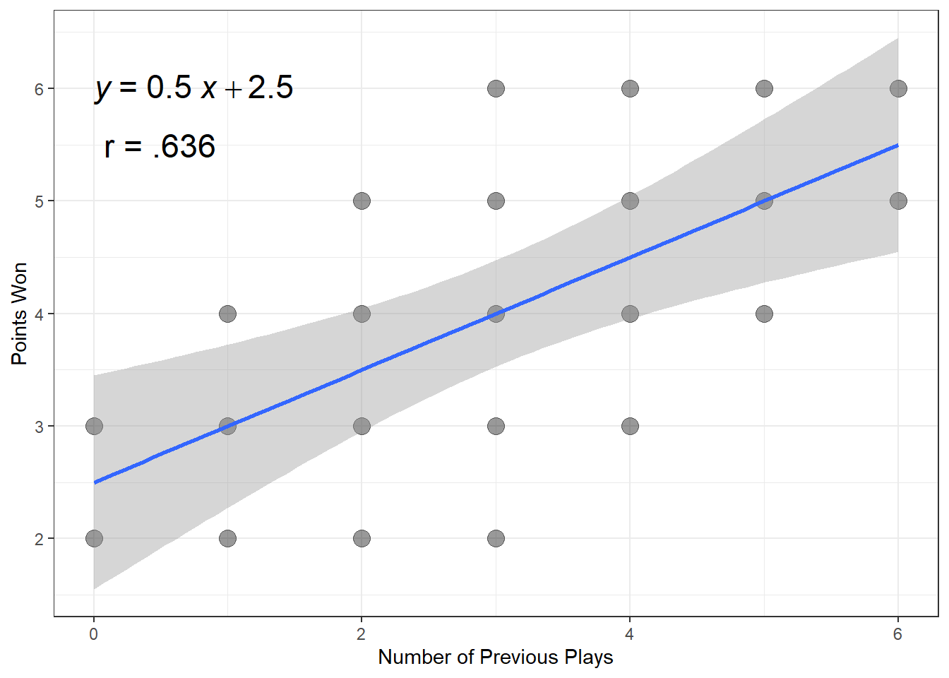
2    21       25      1.19      NA   NA      

2.4.6 Visualize

df_golf %>% 
  ggplot(aes(x = X,
             y = Y)) +
  theme_bw() +
  geom_point(size = 4,
             alpha = .4) +
  geom_smooth(method = "lm",
              formula = y ~ x)  +
  annotate(x = 0.5,
           y = 5.5,
           size = 6,
           geom = "text",
           label = "r = .636") +
  ggpubr::stat_regline_equation(label.x = 0,
                                label.y = 6,
                                size = 6) +
  labs(x = "Number of Previous Plays",
       y = "Points Won")

Figure 2.7
Regress Points Won on Number of Previous Plays

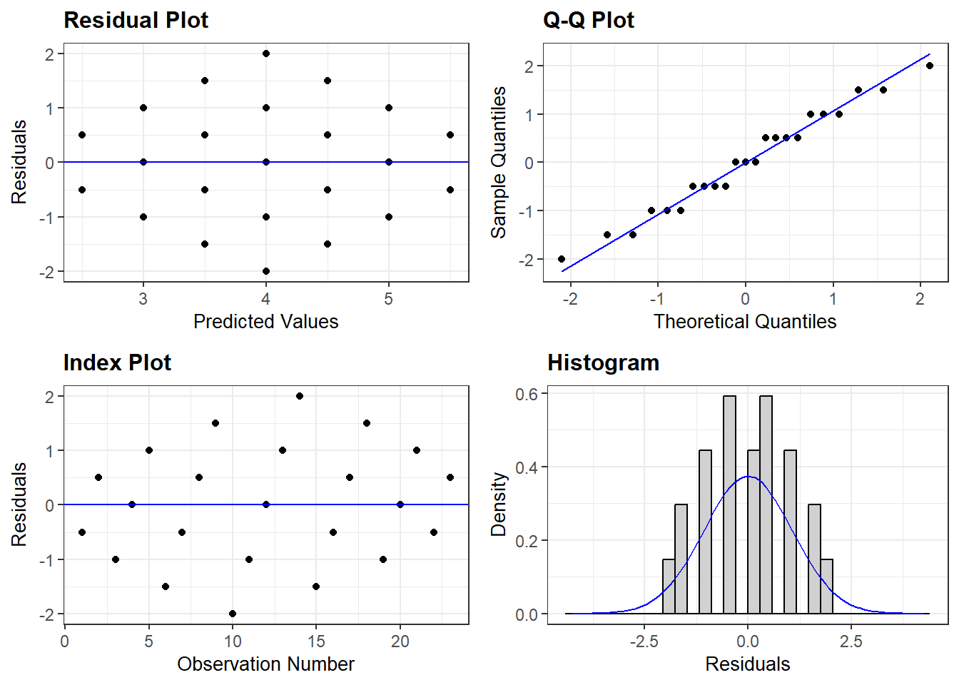
2.5 RESIDUALS

2.5.1 Properties

1. Mean of residuals = zero

summary(fit_lm_golf$residuals)

   Min. 1st Qu.  Median    Mean 3rd Qu.    Max. 
  -2.00   -0.75    0.00    0.00    0.75    2.00 

2. Zero correlation between residuals the X

cor(fit_lm_golf$residuals, df_golf$X)

[1] -7.33757e-17

3. Variance of residuals = Proportion of Variance not Explained

\[ \frac{Var(\text{residuals})}{Var(Y)} = 1 - r^2 \tag{D&H 2.12} \]

var(fit_lm_golf$residuals)/var(df_golf$Y)

[1] 0.5952381

1 - (cor(df_golf$X, df_golf$Y))^2

[1] 0.5952381

2.5.2 Residual Analysis

performance::check_residuals(fit_lm_golf)

OK: Simulated residuals appear as uniformly distributed (p = 0.902).

ggResidpanel::resid_panel(fit_lm_golf)