6 D&H Ch6 - Statistical vs. Experimental Control: “PTSD”

Darlington & Hayes, Chapter 6’s first example

# install.packages("remotes")
# remotes::install_github("sarbearschwartz/apaSupp")
# remotes::install_github("ddsjoberg/gtsummary")
     
library(tidyverse) 
library(flextable)
library(apaSupp)
library(car)
library(rempsyc)
library(parameters)
library(performance)
library(interactions)
library(ggResidpanel)

flextable::set_flextable_defaults(digits = 2)

6.1 PURPOSE

RESEARCH QUESTION:

Does the experimental therapy reduce PTSD symptom severity more than the traditional therapy?

6.1.1 Data Description

Hypothetical study of the effect of a proposed therapy for Post-Traumatic Stress Disorder (PTSD) conducted on 14 military veterans who experienced combat. Half were randomly assigned to experience 6 weeks of proposed therapy (experimental) and the other half received 6 weeks of traditional therapy. Each was pre tested with respect to their PTSD symptoms and an identical post test assessment of their symptoms was administered upon the completion of the therapy.

pre_test symptom severity prior to therapy
post_test symptom severity after therapy
gain symptom severity gain
therapy which therapy was randomly assigned

Manually enter the data set provided on page 44 in Table 3.1

df_ptsd <- tibble::tribble(~id, ~post_test, ~pre_test, ~therapy,
                            1,  2,   1,  1,  
                            2,  4,   3,  1,
                            3,  6,   7,  1,
                            4,  6,  10,  1,
                            5,  9,  13,  1,
                            6, 10,  17,  1,
                            7, 12,  19,  1,
                            8,  6,   1,  0,
                            9,  7,   5,  0,
                           10,  9,   7,  0,
                           11,  9,   9,  0,
                           12, 12,  13,  0,
                           13, 12,  16,  0,
                           14, 15,  19,  0) %>% 
  dplyr::mutate(therapy = factor(therapy,
                                 levels = c(0, 1),
                                 labels = c("Traditional", "Experimental"))) %>% 
  dplyr::mutate(gain = post_test - pre_test)

df_ptsd %>% 
  dplyr::select("ID" = id,
                "Therapy"   = therapy,
                "Pre Test"  = pre_test,
                "Post Test" = post_test,
                "Gain"      = gain) %>% 
  flextable::flextable() %>% 
  apaSupp::theme_apa(caption = "Dataset, wide Format") %>% 
  flextable::colformat_double(digits = 0)

``` ```{=html}

(\#tab:unnamed-chunk-239)Dataset, wide Format
ID	Therapy	Pre Test	Post Test	Gain
1	Experimental	1	2	1
2	Experimental	3	4	1
3	Experimental	7	6	-1
4	Experimental	10	6	-4
5	Experimental	13	9	-4
6	Experimental	17	10	-7
7	Experimental	19	12	-7
8	Traditional	1	6	5
9	Traditional	5	7	2
10	Traditional	7	9	2
11	Traditional	9	9	0
12	Traditional	13	12	-1
13	Traditional	16	12	-4
14	Traditional	19	15	-4

6.1.2 Longer Format of Repeated Measures

df_ptsd_long <- df_ptsd %>% 
  dplyr::select(-gain) %>% 
  tidyr::pivot_longer(cols = ends_with("test"),
                      names_to = c("time", ".value"),
                      names_pattern = "(.*)_(.*)") %>% 
  dplyr::mutate(time = factor(time,
                              levels = c("pre", "post"))) %>% 
  dplyr::arrange(id, time)

df_ptsd_long %>% 
  dplyr::select("ID" = id,
                "Therapy"    = therapy,
                "Time"       = time,
                "Test Score" = test) %>% 
  flextable::flextable() %>% 
  apaSupp::theme_apa(caption = "Dataset, Long Format") %>% 
  flextable::colformat_double(digits = 0)

``` ```{=html}

(\#tab:unnamed-chunk-241)Dataset, Long Format
ID	Therapy	Time	Test Score
1	Experimental	pre	1
1	Experimental	post	2
2	Experimental	pre	3
2	Experimental	post	4
3	Experimental	pre	7
3	Experimental	post	6
4	Experimental	pre	10
4	Experimental	post	6
5	Experimental	pre	13
5	Experimental	post	9
6	Experimental	pre	17
6	Experimental	post	10
7	Experimental	pre	19
7	Experimental	post	12
8	Traditional	pre	1
8	Traditional	post	6
9	Traditional	pre	5
9	Traditional	post	7
10	Traditional	pre	7
10	Traditional	post	9
11	Traditional	pre	9
11	Traditional	post	9
12	Traditional	pre	13
12	Traditional	post	12
13	Traditional	pre	16
13	Traditional	post	12
14	Traditional	pre	19
14	Traditional	post	15

6.2 EXPLORATORY DATA ANALYSIS

6.2.1 Descriptive Statistics

6.2.1.1 Univariate

df_ptsd %>% 
  dplyr::select("Therapy" = therapy) %>% 
  apaSupp::tab_freq(caption = "Summary of Categorical Measures")

``` ```{=html}

(\#tab:unnamed-chunk-242)Summary of Categorical Measures
		Statistic (N=14)
Therapy
Traditional		7 (50.0%)
Experimental		7 (50.0%)

df_ptsd %>% 
  dplyr::select("Post Test" = post_test,
                "Pre Test"  = pre_test,
                "Gain" = gain) %>% 
  apaSupp::tab_desc(caption = "Summary of Measures")

``` ```{=html}

(\#tab:unnamed-chunk-243)Summary of Measures
Measure	NA	M	SD	min	Q1	Mdn	Q3	max
Post Test	0	8.50	3.57	2.00	6.00	9.00	11.50	15.00
Pre Test	0	10.00	6.32	1.00	5.50	9.50	15.25	19.00
Gain	0	-1.50	3.59	-7.00	-4.00	-1.00	1.00	5.00
Note. NA = not available or missing. Mdn = median. Q1 = 25th percentile, Q3 = 75th percentile. N = 14.

6.2.1.2 Bivariate

df_ptsd %>% 
  dplyr::select(therapy,
                "Post Test" = post_test,
                "Pre Test"  = pre_test,
                "Gain" = gain) %>% 
  apaSupp::table1_apa(split = therapy,
                      caption = "Descriptive Summary by Therapy Group")

``` ```{=html}

(\#tab:unnamed-chunk-244)Descriptive Summary by Therapy Group
	Total	Traditional	Experimental	p
	n = 14	n = 7	n = 7
Post Test				.119
	8.50 (3.57)	10.00 (3.16)	7.00 (3.51)
Pre Test				1.000
	10.00 (6.32)	10.00 (6.35)	10.00 (6.81)
Gain				.121
	-1.50 (3.59)	0.00 (3.32)	-3.00 (3.42)
Note. Continuous variables summarized by means (standard deviations) and are compared via independent ANOVA.
* p < .05. p < .01. * p < .001.

Pearson’s correlation is only appropriate for TWO CONTINUOUS variables. The exception is when 1 variable is continuous and the other has exactly 2 levels. In this case, the binary variable needs to be converted to two numbers (numeric not factor) and the value is called the Point-Biserial Correlation (\(r_{pb}\)).

df_ptsd %>% 
  dplyr::mutate(therapy = as.numeric(therapy == "Experimental")) %>% 
  dplyr::select("Post Test" = post_test,
                "Pre Test"  = pre_test,
                "Gain" = gain,
                "Therapy" = therapy) %>% 
  apaSupp::tab_cor(caption = "Correlation Between Pairs of Measures",
                   general_note = "For pairs of variables with therapy, r = Point-Biserial Correlation, otherwise ") %>% 
  flextable::hline(i = 3) %>% 
  flextable::bg(i = 1:3, bg = "yellow") %>% 
  flextable::bg(i = c(4), bg = "orange")

``` ```{=html}

(\#tab:unnamed-chunk-246)Correlation Between Pairs of Measures
Variables		r	p
Post Test	Pre Test	0.880	< .001	***
Post Test	Gain	-0.560	.037	*
Post Test	Therapy	-0.440	.119
Pre Test	Gain	-0.880	< .001	***
Pre Test	Therapy	0.000	1.000
Gain	Therapy	-0.430	.121
Note. For pairs of variables with therapy, r = Point-Biserial Correlation, otherwise r = Pearson's Product-Moment correlation coefficient. N = 14.
* p < .05. p < .01. * p < .001.

6.2.2 Visualizing Distributions

6.2.2.1 Univariate

df_ptsd %>% 
  dplyr::mutate(therapy = as.numeric(therapy == "Experimental")) %>% 
  dplyr::select(id,
                "Post Symptom Severity" = post_test,
                "Pre Symptom Severity"  = pre_test,
                "Change in Symptom Severity" = gain,
                "Therapy" = therapy) %>%  
  tidyr::pivot_longer(cols = -id) %>% 
  ggplot(aes(value)) +
  geom_histogram(binwidth = 1,
                 color = "black",
                 alpha = .25) +
  theme_bw() +
  facet_wrap(~ name,
             scale = "free_x") +
  labs(x = NULL,
       y = "Count")

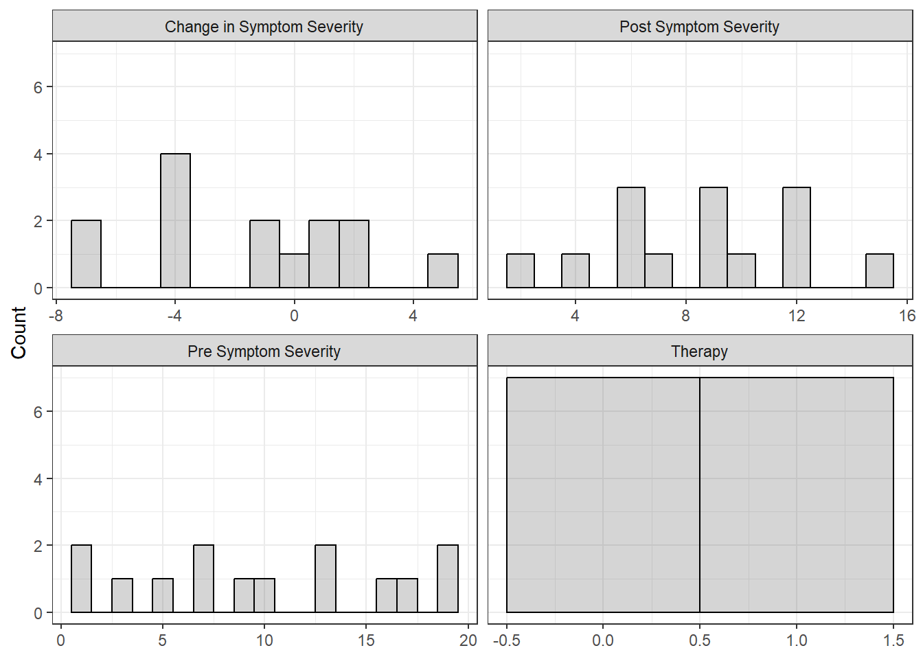
Figure 6.1
Univariate Distibution of Measures

6.2.2.2 Bivariate

apaSupp::spicy_histos(df = df_ptsd,
                      var = pre_test,
                      split = therapy,
                      lab = "Symptom Severity Prior to Therapy") +
  scale_x_continuous(breaks = seq(from = -24, to = 24, by = 2))

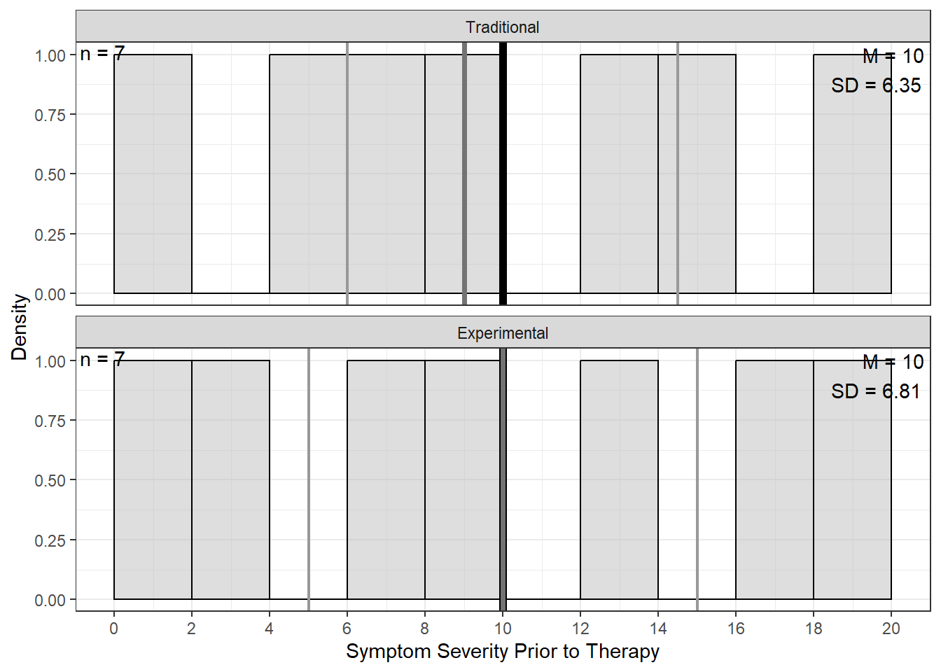
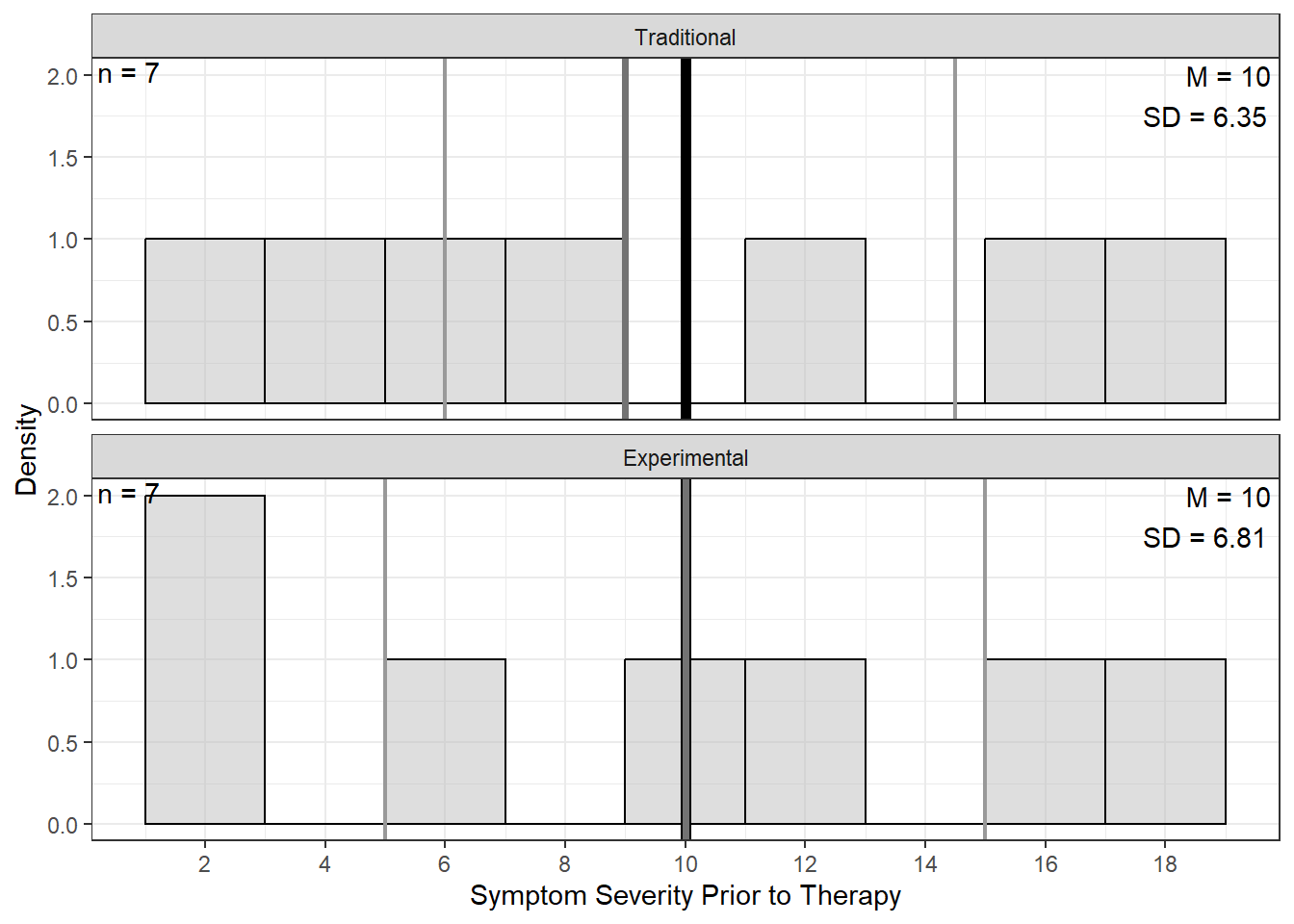
Figure 6.2
Distribution of Symptom Severity Prior to Therapy

apaSupp::spicy_histos(df = df_ptsd,
                      var = post_test,
                      split = therapy,
                      lab = "Symptom Severity After Therapy") +
  scale_x_continuous(breaks = seq(from = -24, to = 24, by = 2))

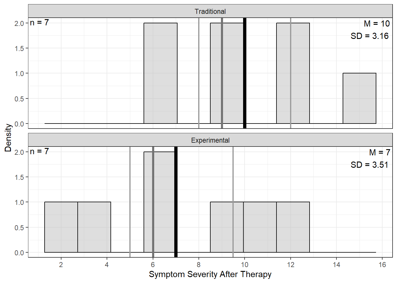
Figure 6.3
Distribution of Symptom Severity After Therapy

apaSupp::spicy_histos(df = df_ptsd,
                      var = gain,
                      split = therapy,
                      lab = "Change in Symptom Severity") +
  scale_x_continuous(breaks = seq(from = -24, to = 24, by = 2))

Figure 6.4
Distribution of Change in Symptom Severity

df_ptsd_long %>% 
  ggplot(aes(x = time,
             y = test,
             group = id)) +
  geom_point() +
  geom_line() +
  theme_bw() +
  labs(x = NULL,
       y = "Symptom Severity Score") +
  facet_grid(~ therapy) +
  stat_summary(aes(group = 1),
           geom = "point",
           fun = "mean",
           shape = 13,
           size = 5,
           color = "red")+
  stat_summary(aes(group = 1),
           geom = "line",
           fun = "mean",
           color = "red",
           linewidth = 1.5)

Figure 6.5
Progression in Symptom Severity, Stratified by Therapy

6.2.2.3 Multivariate

df_ptsd %>% 
  ggplot(aes(x = pre_test,
             y = post_test)) +
  geom_point(aes(color = therapy,
                 shape = therapy),
             size = 3) + 
  theme_bw() +
  geom_smooth(aes(color = therapy,
                  fill = therapy,
                  linetype = therapy),
              method = "lm",
              formula = y ~x,
              alpha = .2) +
  labs(x = "Observed Symptom Severity Prior to Therapy",
       y = "Observed Symptom Severity\nAfter Therapy",
       color    = "Therapy Type:",
       fill     = "Therapy Type:",
       shape    = "Therapy Type:",
       linetype = "Therapy Type:") +
  theme(legend.position.inside = TRUE,
        legend.position = c(0, 1),
        legend.justification = c(-.1, 1.1),
        legend.background = element_rect(color = "black"),
        legend.key.width = unit(2, "cm")) +
  scale_linetype_manual(values = c("solid", "longdash")) +
  scale_x_continuous(breaks = seq(from = 0, to = 24, by = 2)) +
  scale_y_continuous(breaks = seq(from = 0, to = 24, by = 2)) + 
  geom_abline(intercept = 0, slope = 1)

Figure 6.6
Association Between Symptom Severity Prior to and After Therapy, Stratified by Therapy Type

df_ptsd %>% 
  ggplot(aes(x = pre_test,
             y = gain)) +
  geom_point(aes(color = therapy,
                 shape = therapy),
             size = 3) + 
  theme_bw() +
  geom_smooth(aes(color = therapy,
                  fill = therapy,
                  linetype = therapy),
              method = "lm",
              formula = y ~x,
              alpha = .2) +
  labs(x = "Observed Symptom Severity Prior to Therapy",
       y = "Observed Change in Symptom Severity",
       color    = "Therapy Type:",
       fill     = "Therapy Type:",
       shape    = "Therapy Type:",
       linetype = "Therapy Type:") +
  theme(legend.position.inside = TRUE,
        legend.position = c(1, 1),
        legend.justification = c(1.1, 1.1),
        legend.background = element_rect(color = "black"),
        legend.key.width = unit(2, "cm")) +
  scale_linetype_manual(values = c("solid", "longdash")) +
  scale_x_continuous(breaks = seq(from = 0, to = 24, by = 2))+
  scale_y_continuous(breaks = seq(from = -24, to = 24, by = 2)) +
  geom_hline(yintercept = 0)

Figure 6.7
Association Between Test Gain in Score and Pre-Test, Stratified by Therapy

6.3 REGRESSION ANALYSIS

6.3.1 DV = Post Score, controlling for Pre Score

fit_ptsd_1 <- lm(post_test ~ pre_test + therapy,
                 data = df_ptsd)

summary(fit_ptsd_1)


Call:
lm(formula = post_test ~ pre_test + therapy, data = df_ptsd)

Residuals:
    Min      1Q  Median      3Q     Max 
-1.0000 -0.5077  0.4846  0.5029  0.5173 

Coefficients:
                    Estimate Std. Error t value Pr(>|t|)    
(Intercept)          5.01923    0.39024  12.862 5.68e-08 ***
pre_test             0.49808    0.02956  16.850 3.33e-09 ***
therapyExperimental -3.00000    0.36031  -8.326 4.46e-06 ***
---
Signif. codes:  0 '***' 0.001 '**' 0.01 '*' 0.05 '.' 0.1 ' ' 1

Residual standard error: 0.6741 on 11 degrees of freedom
Multiple R-squared:  0.9698,    Adjusted R-squared:  0.9643 
F-statistic: 176.6 on 2 and 11 DF,  p-value: 4.365e-09

anova(fit_ptsd_1)

# A tibble: 3 × 5
     Df `Sum Sq` `Mean Sq` `F value` `Pr(>F)`
  <int>    <dbl>     <dbl>     <dbl>    <dbl>
1     1   129.     129.        284.   3.33e-9
2     1    31.5     31.5        69.3  4.46e-6
3    11     5.00     0.454      NA   NA

6.3.1.1 Equation

\[ \widehat{post} = 5.019 + 0.498(pre) -3.00(type=exp) \]

6.3.1.2 Role of Therapy

Test the significance for therapy: t(11) = -8.33, p <.001, VERY significant

After controlling for pre-test score, the experimental therapy is associated with 3 point lower post-test score compared to the traditional therapy, b = -3.00, SE = 0.36, p <.001.

Notes:

Covariate pre_test has b = -0.50, SE = 0.03, p <.001.

The entire model: SSresid = 4.998, R^2 = .970, F(2, 11) = 176.6, p < .001

6.3.2 DV = Gain Score, ignoring Pre-Score

fit_ptsd_2 <- lm(gain ~ therapy,
                 data = df_ptsd)

summary(fit_ptsd_2)


Call:
lm(formula = gain ~ therapy, data = df_ptsd)

Residuals:
   Min     1Q Median     3Q    Max 
 -4.00  -3.25  -0.50   2.00   5.00 

Coefficients:
                      Estimate Std. Error t value Pr(>|t|)
(Intercept)         -7.121e-16  1.272e+00   0.000    1.000
therapyExperimental -3.000e+00  1.799e+00  -1.667    0.121

Residual standard error: 3.367 on 12 degrees of freedom
Multiple R-squared:  0.1881,    Adjusted R-squared:  0.1204 
F-statistic: 2.779 on 1 and 12 DF,  p-value: 0.1213

anova(fit_ptsd_2)

# A tibble: 2 × 5
     Df `Sum Sq` `Mean Sq` `F value` `Pr(>F)`
  <int>    <dbl>     <dbl>     <dbl>    <dbl>
1     1     31.5      31.5      2.78    0.121
2    12    136        11.3     NA      NA

6.3.2.1 Equation

\[ \widehat{gain} = 0 -3.00(EXP) \]

6.3.2.2 Role of Therapy

Test the significance for therapy: t(12) = -1.67, p = .121, NOT significant

No evidence was found that the therapy type was associated with a differential change in symptom severity,b = -3.00, SE = 1.80, p =.121.

Note:

The entire model: SSresid = 136, R^2 = .188, F(1, 11) = 2.78, p =.121

6.3.2.3 Equivalent Analysis: independent groups t-test

t.test(gain ~ therapy,
       data = df_ptsd)


    Welch Two Sample t-test

data:  gain by therapy
t = 1.6672, df = 11.99, p-value = 0.1214
alternative hypothesis: true difference in means between group Traditional and group Experimental is not equal to 0
95 percent confidence interval:
 -0.9210863  6.9210863
sample estimates:
 mean in group Traditional mean in group Experimental 
                         0                         -3

6.3.3 DV = Gain Score, controlling for Pre-Score

fit_ptsd_3 <- lm(gain ~ pre_test + therapy,
                 data = df_ptsd)

summary(fit_ptsd_3)


Call:
lm(formula = gain ~ pre_test + therapy, data = df_ptsd)

Residuals:
    Min      1Q  Median      3Q     Max 
-1.0000 -0.5077  0.4846  0.5029  0.5173 

Coefficients:
                    Estimate Std. Error t value Pr(>|t|)    
(Intercept)          5.01923    0.39024  12.862 5.68e-08 ***
pre_test            -0.50192    0.02956 -16.980 3.07e-09 ***
therapyExperimental -3.00000    0.36031  -8.326 4.46e-06 ***
---
Signif. codes:  0 '***' 0.001 '**' 0.01 '*' 0.05 '.' 0.1 ' ' 1

Residual standard error: 0.6741 on 11 degrees of freedom
Multiple R-squared:  0.9702,    Adjusted R-squared:  0.9647 
F-statistic: 178.8 on 2 and 11 DF,  p-value: 4.086e-09

anova(fit_ptsd_3)

# A tibble: 3 × 5
     Df `Sum Sq` `Mean Sq` `F value` `Pr(>F)`
  <int>    <dbl>     <dbl>     <dbl>    <dbl>
1     1   131.     131.        288.   3.07e-9
2     1    31.5     31.5        69.3  4.46e-6
3    11     5.00     0.454      NA   NA

6.3.3.1 Equation

\[ \widehat{gain} = 5.019 - 0.50(pre) -3.00(EXP) \]

6.3.3.2 Role of Therapy

Test the significance for therapy type on symptom severity change: t(11) = -8.33, p <.001, VERY significant

After controlling for symptom severity prior to therapy, the experimental therapy was associated with 3 point lower change on symptom severity after therapy compared to traditional therapy, b = -3.00, SE = 0.36, p <.001.

Notes:

Covariate pre_test has b = -0.50, SE = 0.03, p <.001.

The entire model: SSresid = 4.998, R^2 = .970, F(2, 11) = 178.8, p < .001

6.3.4 Compare Models

performance::compare_performance(fit_ptsd_1, fit_ptsd_2, fit_ptsd_3,
                                 metrics = c("AIC", "BIC",
                                             "R2", "R2_adj",
                                             "RMSE", "SIGMA"))

# A tibble: 3 × 10
  Name       Model   AIC   AIC_wt   BIC   BIC_wt    R2 R2_adjusted  RMSE Sigma
  <chr>      <chr> <dbl>    <dbl> <dbl>    <dbl> <dbl>       <dbl> <dbl> <dbl>
1 fit_ptsd_1 lm     33.3 5.00e- 1  35.9 5.00e- 1 0.970       0.964 0.597 0.674
2 fit_ptsd_2 lm     77.6 1.23e-10  79.5 1.69e-10 0.188       0.120 3.12  3.37 
3 fit_ptsd_3 lm     33.3 5.00e- 1  35.9 5.00e- 1 0.970       0.965 0.597 0.674

6.4 ALTERNATIVE ANALYSIS

6.4.1 2x2 mix ANOVA

fit_aov <- afex::aov_4(test ~ therapy + (time|id),
                       data = df_ptsd_long)

summary(fit_aov)


Univariate Type III Repeated-Measures ANOVA Assuming Sphericity

              Sum Sq num Df Error SS den Df F value    Pr(>F)    
(Intercept)  2395.75      1      586     12 49.0597 1.426e-05 ***
therapy        15.75      1      586     12  0.3225    0.5806    
time           15.75      1       68     12  2.7794    0.1213    
therapy:time   15.75      1       68     12  2.7794    0.1213    
---
Signif. codes:  0 '***' 0.001 '**' 0.01 '*' 0.05 '.' 0.1 ' ' 1