9 D&H Ch9 - Multicategorical Regressors: “married”

Compiled: September 18, 2025

Darlington & Hayes, Chapter 9’s example

# install.packages("remotes")
# remotes::install_github("sarbearschwartz/apaSupp") # 9/17/2025

library(haven)
library(tidyverse)   
library(flextable)
library(apaSupp)       # not on CRAN, get from GitHub (above) 
library(GGally)
library(afex)
library(emmeans)
library(interactions) 

9.1 PURPOSE

RESEARCH QUESTION:

RQ 1) Does life satisfaction differ by marital status?

RQ2) Is there an association between income and life satisfaction, after controlling for marital status?

9.1.1 Data Import

You can download the married dataset here:

• SPSS format (.sav)

df_spss <- haven::read_sav("married.sav")

tibble::glimpse(df_spss)

Rows: 20
Columns: 4
$ mstatus <dbl+lbl> 3, 2, 4, 4, 1, 3, 2, 2, 3, 1, 3, 4, 1, 1, 2, 1, 3, 2, 4, 1
$ satis   <dbl> 85, 80, 72, 60, 92, 88, 74, 84, 88, 82, 76, 78, 78, 93, 73…
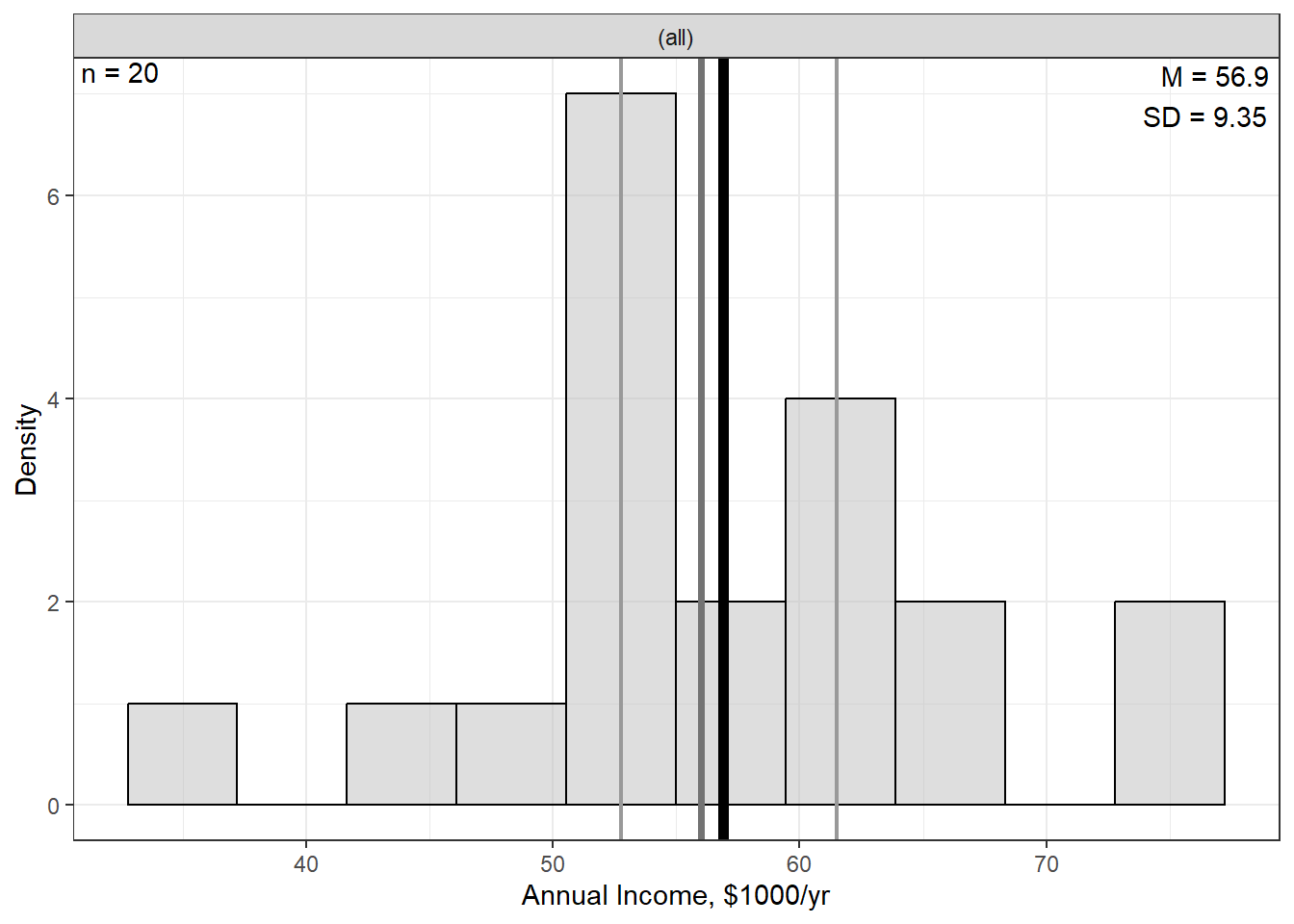
$ income  <dbl> 53, 65, 54, 35, 73, 75, 57, 59, 60, 52, 47, 60, 63, 66, 51, 53…
$ sex     <dbl+lbl> 0, 1, 0, 0, 1, 1, 0, 0, 0, 0, 1, 0, 1, 1, 0, 1, 0, 1, 0, 1

summary(df_spss)

    mstatus         satis           income           sex      
 Min.   :1.00   Min.   :60.00   Min.   :35.00   Min.   :0.00  
 1st Qu.:1.00   1st Qu.:75.75   1st Qu.:52.75   1st Qu.:0.00  
 Median :2.00   Median :80.00   Median :56.00   Median :0.00  
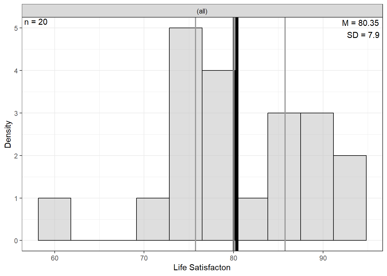
 Mean   :2.35   Mean   :80.35   Mean   :56.90   Mean   :0.45  
 3rd Qu.:3.00   3rd Qu.:85.75   3rd Qu.:61.50   3rd Qu.:1.00  
 Max.   :4.00   Max.   :93.00   Max.   :75.00   Max.   :1.00  

When importing data from SPSS (.sav), you need to be careful how categorical vairables are stored.

df_fac <- df_spss %>% 
  haven::as_factor()

tibble::glimpse(df_fac)

Rows: 20
Columns: 4
$ mstatus <fct> single, divorced, widowed, widowed, married, single, divorced,…
$ satis   <dbl> 85, 80, 72, 60, 92, 88, 74, 84, 88, 82, 76, 78, 78, 93, 73, 80…
$ income  <dbl> 53, 65, 54, 35, 73, 75, 57, 59, 60, 52, 47, 60, 63, 66, 51, 53…
$ sex     <fct> female, male, female, female, male, male, female, female, fema…

summary(df_fac)

     mstatus      satis           income          sex    
 married :6   Min.   :60.00   Min.   :35.00   female:11  
 divorced:5   1st Qu.:75.75   1st Qu.:52.75   male  : 9  
 single  :5   Median :80.00   Median :56.00              
 widowed :4   Mean   :80.35   Mean   :56.90              
              3rd Qu.:85.75   3rd Qu.:61.50              
              Max.   :93.00   Max.   :75.00              

9.1.2 Data Description

9.1.2.1 Variables

Dependent Variable (outcome, Y)

• statis life satisfaction, scale 1-100 (composite of many items)

Independent Variables (predictors or regressors, X’s)

• mstatus marital status: 1 = married, 2 = divorced, 3 = single, 4 = widowed
  
• income annual income, $1000s/year
  
• sex 0 = female, 1 = male

Categorical variables MUST be declare as FACTORS and the FIRST level listed is treated as the reference category.

df_sat <- df_spss %>% 
  haven::as_factor() %>% 
  tibble::rowid_to_column(var = "id") %>% 
  dplyr::mutate(mstatus = forcats::fct_recode(mstatus,
                                              "Married"  = "married",
                                              "Divorced" = "divorced",
                                              "Single"   = "single",
                                              "Widowed"  = "widowed")) %>% 
  dplyr::mutate(sex = forcats::fct_recode(sex,
                                          "Female" = "female",
                                          "Male" = "male")) %>% 
  dplyr::mutate(mstat_mar = forcats::fct_relevel(mstatus, "Married",  after = 0)) %>%
  dplyr::mutate(mstat_div = forcats::fct_relevel(mstatus, "Divorced", after = 0)) %>% 
  dplyr::mutate(mstat_sin = forcats::fct_relevel(mstatus, "Single",   after = 0)) %>% 
  dplyr::mutate(mstat_wid = forcats::fct_relevel(mstatus, "Widowed",  after = 0)) %>% 
  dplyr::mutate(male   = forcats::fct_relevel(sex, "Male",   after = 1)) %>% 
  dplyr::mutate(female = forcats::fct_relevel(sex, "Female", after = 1))

tibble::glimpse(df_sat)

Rows: 20
Columns: 11
$ id        <int> 1, 2, 3, 4, 5, 6, 7, 8, 9, 10, 11, 12, 13, 14, 15, 16, 17, 1…
$ mstatus   <fct> Single, Divorced, Widowed, Widowed, Married, Single, Divorce…
$ satis     <dbl> 85, 80, 72, 60, 92, 88, 74, 84, 88, 82, 76, 78, 78, 93, 73, …
$ income    <dbl> 53, 65, 54, 35, 73, 75, 57, 59, 60, 52, 47, 60, 63, 66, 51, …
$ sex       <fct> Female, Male, Female, Female, Male, Male, Female, Female, Fe…
$ mstat_mar <fct> Single, Divorced, Widowed, Widowed, Married, Single, Divorce…
$ mstat_div <fct> Single, Divorced, Widowed, Widowed, Married, Single, Divorce…
$ mstat_sin <fct> Single, Divorced, Widowed, Widowed, Married, Single, Divorce…
$ mstat_wid <fct> Single, Divorced, Widowed, Widowed, Married, Single, Divorce…
$ male      <fct> Female, Male, Female, Female, Male, Male, Female, Female, Fe…
$ female    <fct> Female, Male, Female, Female, Male, Male, Female, Female, Fe…

summary(df_sat)

       id            mstatus      satis           income          sex    
 Min.   : 1.00   Married :6   Min.   :60.00   Min.   :35.00   Female:11  
 1st Qu.: 5.75   Divorced:5   1st Qu.:75.75   1st Qu.:52.75   Male  : 9  
 Median :10.50   Single  :5   Median :80.00   Median :56.00              
 Mean   :10.50   Widowed :4   Mean   :80.35   Mean   :56.90              
 3rd Qu.:15.25                3rd Qu.:85.75   3rd Qu.:61.50              
 Max.   :20.00                Max.   :93.00   Max.   :75.00              
    mstat_mar    mstat_div    mstat_sin    mstat_wid     male       female  
 Married :6   Divorced:5   Single  :5   Widowed :4   Female:11   Male  : 9  
 Divorced:5   Married :6   Married :6   Married :6   Male  : 9   Female:11  
 Single  :5   Single  :5   Divorced:5   Divorced:5                          
 Widowed :4   Widowed :4   Widowed :4   Single  :5                          
                                                                            
                                                                            

9.2 EXPLORATORY DATA ANALYSIS

Before embarking on any inferencial anlaysis or modeling, always get familiar with your variables one at a time (univariate), as well as pairwise (bivariate).

9.2.1 Summary Statistics

9.2.1.1 Univariate

df_sat %>% 
  dplyr::select("Sex" = sex,
                "Marital Status" = mstatus) %>% 
  apaSupp::tab_freq(caption = "Description of Categorical Measures")

Table 9.1
Description of Categorical Measures

		Statistic (N=20)
Sex
Female		11 (55.0%)
Male		9 (45.0%)
Marital Status
Married		6 (30.0%)
Divorced		5 (25.0%)
Single		5 (25.0%)
Widowed		4 (20.0%)

df_sat %>% 
  dplyr::select("Annual Income" = income,
                "Life Satisfaction" = satis) %>% 
  apaSupp::tab_desc(caption = "Description of Continuous Measures",
                    general_note = "Annual income is in $1000s per year.  Life Satisfaction is a composite score on a scale 1-100.")

Table 9.2
Description of Continuous Measures

	NA	M	SD	min	Q1	Mdn	Q3	max
Annual Income	0	56.90	9.35	35.00	52.75	56.00	61.50	75.00
Life Satisfaction	0	80.35	7.90	60.00	75.75	80.00	85.75	93.00
Note. N = 20. NA = not available or missing; Mdn = median; Q1 = 25th percentile; Q3 = 75th percentile. Annual income is in $1000s per year. Life Satisfaction is a composite score on a scale 1-100.

9.2.1.2 Bivariate

df_sat %>% 
  dplyr::select(mstatus,
                "Sex" = sex,
                "Annual Income" = income,
                "Life Satisfaction" = satis) %>% 
  apaSupp::tab1(split = "mstatus",
                total_last = FALSE,
                caption = "Description of Continuous Measures",
                general_note = "Annual income is in $1000s per year.  Life Satisfaction is a composite score on a scale 1-100.")

Table 9.3
Description of Continuous Measures

	Total N = 20	Married n = 6 (30.0%)	Divorced n = 5 (25.0%)	Single n = 5 (25.0%)	Widowed n = 4 (20.0%)	p-value
Sex						.074
Female	11 (55.0%)	1 (16.7%)	3 (60.0%)	3 (60.0%)	4 (100.0%)
Male	9 (45.0%)	5 (83.3%)	2 (40.0%)	2 (40.0%)	0 (0.0%)
Annual Income	56.90 (9.35)	60.33 (8.38)	58.60 (5.18)	55.80 (12.36)	51.00 (10.98)	.600
Life Satisfaction	80.35 (7.90)	85.50 (6.38)	79.20 (5.54)	82.40 (6.43)	71.50 (8.06)	.117
Note. Continuous variables are summarized with means (SD) and significant group differences assessed via independent one-way analysis of vaiance (ANOVA). Categorical variables are summarized with counts (%) and significant group differences assessed via Chi-squared tests for independence. Annual income is in $1000s per year. Life Satisfaction is a composite score on a scale 1-100.
* p < .05. ** p < .01. *** p < .001.

cor.test(~ satis + income, data = df_sat)

    Pearson's product-moment correlation

data:  satis and income
t = 4.8906, df = 18, p-value = 0.0001177
alternative hypothesis: true correlation is not equal to 0
95 percent confidence interval:
 0.4699333 0.8977898
sample estimates:
      cor 
0.7553708 

9.2.2 Visualize Distributions

9.2.2.1 Univariate

Always plot your data first!

df_sat %>% 
  apaSupp::spicy_histos(var = satis,
                        lab = "Life Satisfacton")

df_sat %>% 
  apaSupp::spicy_histos(var = income,
                        lab = "Annual Income, $1000/yr")

9.2.2.2 Bivariate

df_sat %>% 
  dplyr::select("Life Satisfaction" = satis,
                "Income" = income,
                "Marital Satus" = mstatus,
                "Sex" = sex) %>%
  data.frame %>% 
  GGally::ggpairs() +
  theme_bw()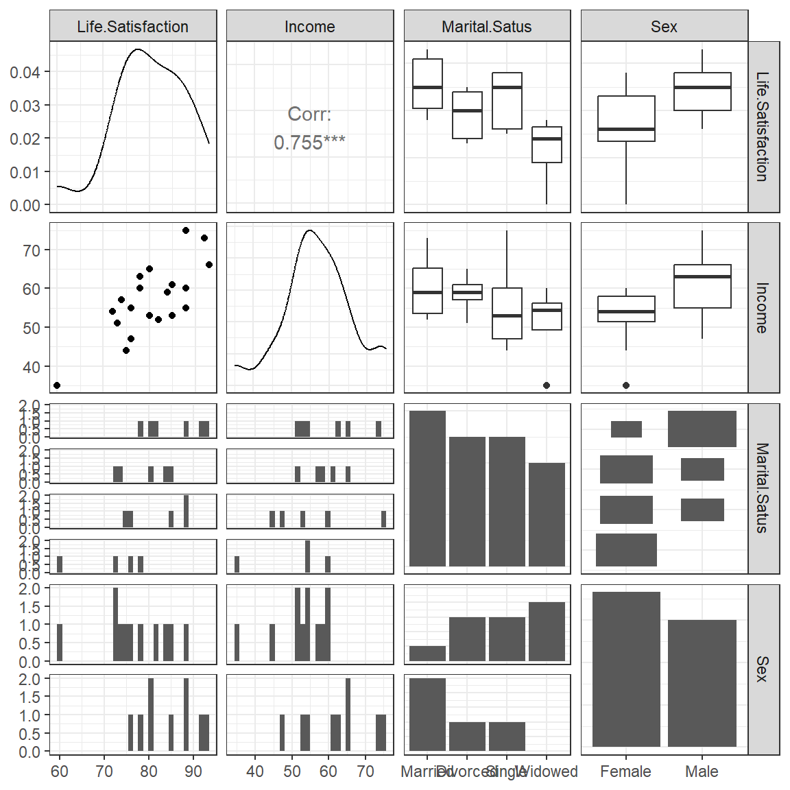

df_sat %>% 
  apaSupp::spicy_histos(var = satis,
                        split = mstatus,
                        lab = "Life Satisfacton")

df_sat %>% 
  ggplot(aes(x = mstatus,
             y = satis,
             group = mstatus)) +
  geom_violin(fill = "gray") +
  geom_boxplot(width = .25) +
  geom_point(color = "red",
             position = position_jitter(width = .1),
             size = 2) +
  theme_bw() +
  labs(x = "Marital Status",
       y = "Observed Life Satisfaction")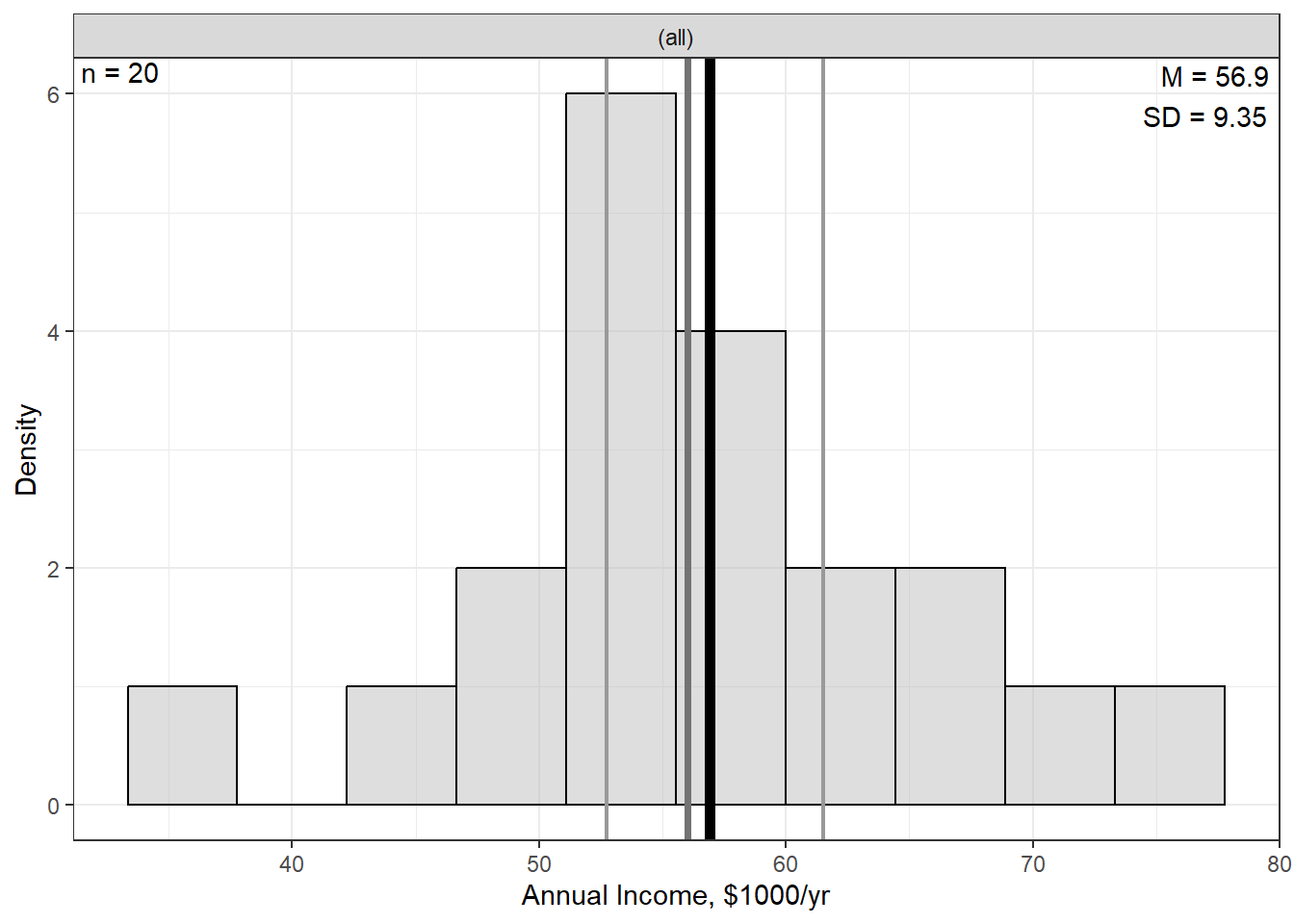

df_sat %>% 
  apaSupp::spicy_histos(var = satis,
                        split = sex,
                        lab = "Life Satisfacton")

df_sat %>% 
  ggplot(aes(x = sex,
             y = satis,
             group = sex)) +
  geom_violin(fill = "gray") +
  geom_boxplot(width = .25) +
  geom_point(color = "red",
             position = position_jitter(width = .1),
             size = 2) +
  theme_bw() +
  labs(x = NULL,
       y = "Observed Life Satisfaction")

df_sat %>% 
  ggplot(aes(x = income,
             y = satis)) +
  geom_point(aes(color = mstatus,
                 shape = mstatus),
             size = 2) +
  theme_bw() +
  geom_smooth(method = "lm",
              formula = y ~ x,
              color = "gray",
              alpha = .2) +
  labs(x = "Annual Income, $1000/yr",
       y = "Observed Life Satisfaction, 1-100",
       color = NULL,
       shape = NULL) +
  theme(legend.position = c(0, 1),
        legend.justification = c(-.1, 1.1),
        legend.background = element_rect(color = "black"))

df_sat %>% 
  ggplot(aes(x = income,
             y = satis)) +
  geom_point() +
  theme_bw() +
  geom_smooth(method = "lm",
              formula = y ~ x,
              alpha = .2) +
  labs(x = "Annual Income, $1000/yr",
       y = "Observed Life Satisfaction") +
  facet_wrap(~ mstatus)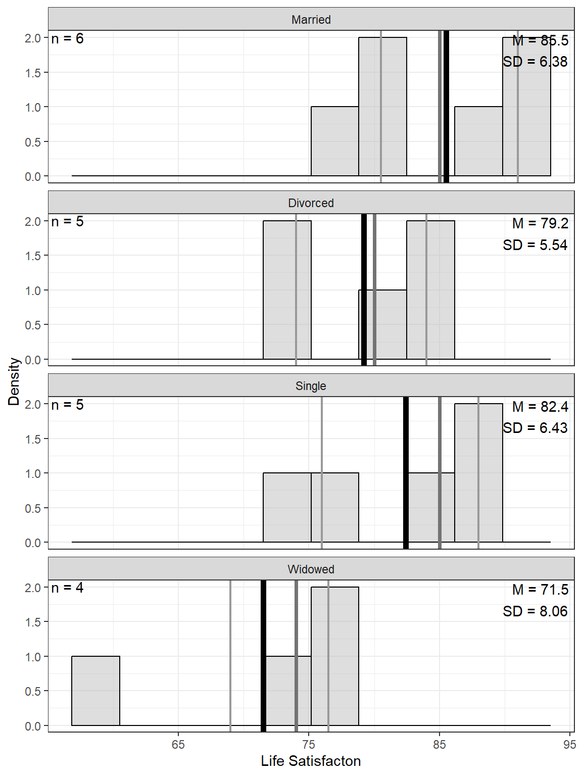

df_sat %>% 
  ggplot(aes(x = income,
             y = satis)) +
  geom_point(aes(color = mstatus,
                 shape = mstatus),
             size = 2) +
  theme_bw() +
  geom_smooth(aes(color = mstatus),
              method = "lm",
              formula = y ~ x,
              se = FALSE) +
  labs(x = "Annual Income, $1000/yr",
       y = "Observed Life Satisfaction, 1-100",
       color = NULL,
       shape = NULL) +
  theme(legend.position = c(0, 1),
        legend.justification = c(-.1, 1.1),
        legend.background = element_rect(color = "black"))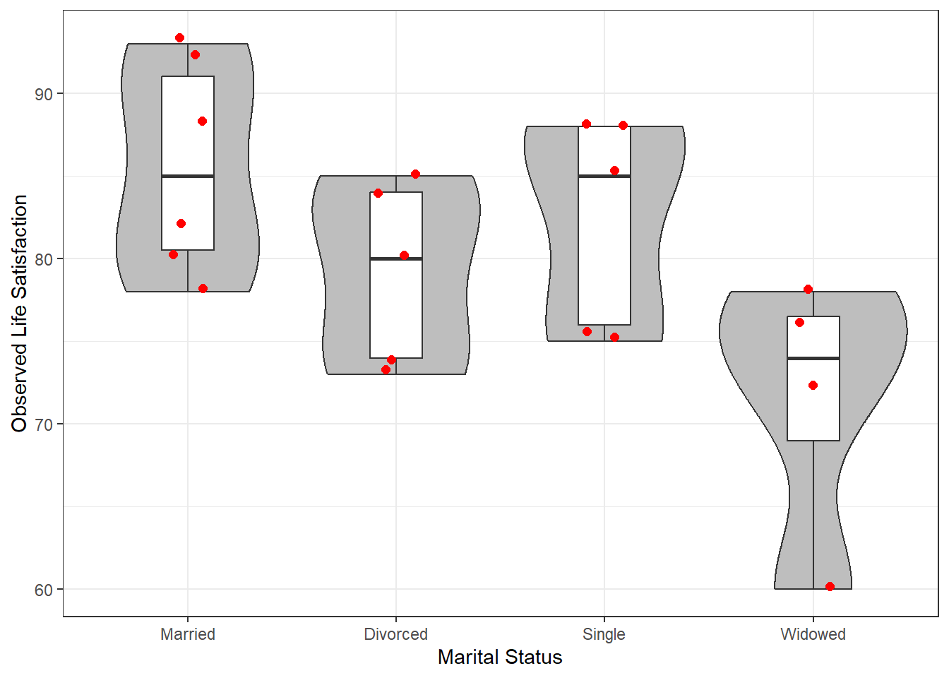

df_sat %>% 
  ggplot(aes(x = income,
             y = satis)) +
  geom_point(aes(color = sex,
                 shape = sex),
             size = 2) +
  theme_bw() +
  geom_smooth(aes(color = sex),
              method = "lm",
              formula = y ~ x,
              alpha = .2) +
  labs(x = "Annual Income, $1000/yr",
       y = "Observed Life Satisfaction, 1-100",
       color = NULL,
       shape = NULL) +
  theme(legend.position = c(0, 1),
        legend.justification = c(-.1, 1.1),
        legend.background = element_rect(color = "black"))

9.3 ANALYSIS OF VARIANE

• The dependent variable (DV) is Life Satisfaction (\(satis\))

9.3.1 By Marital Status

• The independent variable (IV) is marital status, with widowed as the reference category to match the textbook.

NOTE: SPSS used the LAST listed category level as the reference group whereas R uses the FIRST.

fit_aov_1 <- afex::aov_4(satis ~ mstat_wid + (1|id), 
                         data = df_sat)

summary(fit_aov_1)

# A tibble: 1 × 6
  `num Df` `den Df`   MSE     F   ges `Pr(>F)`
     <dbl>    <dbl> <dbl> <dbl> <dbl>    <dbl>
1        3       16  42.9  3.88 0.421   0.0292

fit_aov_1 %>% 
  emmeans::emmeans(~ mstat_wid)

 mstat_wid emmean   SE df lower.CL upper.CL
 Widowed     71.5 3.28 16     64.6     78.4
 Married     85.5 2.67 16     79.8     91.2
 Divorced    79.2 2.93 16     73.0     85.4
 Single      82.4 2.93 16     76.2     88.6

Confidence level used: 0.95 

fit_aov_1 %>% 
  emmeans::emmeans(~ mstat_wid) %>% 
  pairs()

 contrast           estimate   SE df t.ratio p.value
 Widowed - Married     -14.0 4.23 16  -3.311  0.0207
 Widowed - Divorced     -7.7 4.39 16  -1.752  0.3308
 Widowed - Single      -10.9 4.39 16  -2.481  0.1015
 Married - Divorced      6.3 3.97 16   1.588  0.4123
 Married - Single        3.1 3.97 16   0.782  0.8617
 Divorced - Single      -3.2 4.14 16  -0.772  0.8657

P value adjustment: tukey method for comparing a family of 4 estimates 

9.3.2 By Sex

• The independent variable (IV) is sex.

fit_aov_2 <- afex::aov_4(satis ~ sex + (1|id), 
                         data = df_sat)

summary(fit_aov_2)

# A tibble: 1 × 6
  `num Df` `den Df`   MSE     F   ges `Pr(>F)`
     <dbl>    <dbl> <dbl> <dbl> <dbl>    <dbl>
1        1       18  50.7  5.41 0.231   0.0319

9.4 REGRESSION ANALYSIS

• The dependent variable (DV) is Life Satisfaction (\(satis\))

9.4.1 Roll of Marital Status

fit_lm_1 <- lm(satis ~ mstat_wid, data = df_sat)

apaSupp::tab_lm(fit_lm_1, 
                var_labels = c(mstat_wid = "Marital Status"),
                caption = "Parameter Estimates for Life Satisfaction Regressed on Marital Status")

Table 9.4
Parameter Estimates for Life Satisfaction Regressed on Marital Status

	b	(SE)	p	$b^*$	$\eta^2$	$\eta^2_p$
(Intercept)	71.50	(3.28)	< .001***
Marital Status					.421	.421
Widowed	—	—
Married	14.00	(4.23)	.004**
Divorced	7.70	(4.39)	.099
Single	10.90	(4.39)	.025*
R²	.421
Adjusted R²	.313
Note. N = 20. $b^*$ = standardize coefficient; $\eta^2$ = semi-partial correlation; $\eta^2_p$ = partial correlation; p = significance from Wald t-test for parameter estimate.
* p < .05. ** p < .01. *** p < .001.

anova(fit_lm_1)

# A tibble: 2 × 5
     Df `Sum Sq` `Mean Sq` `F value` `Pr(>F)`
  <int>    <dbl>     <dbl>     <dbl>    <dbl>
1     3     500.     167.       3.88   0.0292
2    16     686.      42.9     NA     NA     

fit_lm_1 %>% 
  emmeans::emmeans(~ mstat_wid)

 mstat_wid emmean   SE df lower.CL upper.CL
 Widowed     71.5 3.28 16     64.6     78.4
 Married     85.5 2.67 16     79.8     91.2
 Divorced    79.2 2.93 16     73.0     85.4
 Single      82.4 2.93 16     76.2     88.6

Confidence level used: 0.95 

fit_lm_1 %>% 
  emmeans::emmeans(~ mstat_wid) %>% 
  pairs()

 contrast           estimate   SE df t.ratio p.value
 Widowed - Married     -14.0 4.23 16  -3.311  0.0207
 Widowed - Divorced     -7.7 4.39 16  -1.752  0.3308
 Widowed - Single      -10.9 4.39 16  -2.481  0.1015
 Married - Divorced      6.3 3.97 16   1.588  0.4123
 Married - Single        3.1 3.97 16   0.782  0.8617
 Divorced - Single      -3.2 4.14 16  -0.772  0.8657

P value adjustment: tukey method for comparing a family of 4 estimates 

9.4.1.1 Change the Reference Category

fit_lm_1m <- lm(satis ~ mstat_mar, data = df_sat)
fit_lm_1d <- lm(satis ~ mstat_div, data = df_sat)
fit_lm_1s <- lm(satis ~ mstat_sin, data = df_sat)
fit_lm_1w <- lm(satis ~ mstat_wid, data = df_sat)

apaSupp::tab_lms(list(fit_lm_1m, fit_lm_1d, fit_lm_1s, fit_lm_1w),
                 var_labels = c(mstat_mar = "Marital Status",
                                mstat_div = "Marital Status",
                                mstat_sin = "Marital Status",
                                mstat_wid = "Marital Status"),
                 caption = "Comparison of Regression Models Changing the Reference Category",
                 d = 1,
                 narrow = TRUE)

Table 9.5
Comparison of Regression Models Changing the Reference Category

	Model 1		Model 2		Model 3		Model 4
Variable	b	(SE)	b	(SE)	b	(SE)	b	(SE)
(Intercept)	85.5	(2.7) ***	79.2	(2.9) ***	82.4	(2.9) ***	71.5	(3.3) ***
Marital Status
Married	—	—
Divorced	-6.3	(4.0)
Single	-3.1	(4.0)
Widowed	-14.0	(4.2) **
Marital Status
Divorced			—	—
Married			6.3	(4.0)
Single			3.2	(4.1)
Widowed			-7.7	(4.4)
Marital Status
Single					—	—
Married					3.1	(4.0)
Divorced					-3.2	(4.1)
Widowed					-10.9	(4.4) *
Marital Status
Widowed							—	—
Married							14.0	(4.2) **
Divorced							7.7	(4.4)
Single							10.9	(4.4) *
AIC	137.5		137.5		137.5		137.5
BIC	142.5		142.5		142.5		142.5
R²	.42		.42		.42		.42
Adjusted R²	.31		.31		.31		.31
Note.
* p < .05. ** p < .01. *** p < .001.

9.4.2 Roll of Income

9.4.2.1 Unadjusted Model

No Covariates

fit_lm_2 <- lm(satis ~ income, data = df_sat)

apaSupp::tab_lm(fit_lm_2)

Table 9.6
Parameter Estimates for Linear Regression

	b	(SE)	p	$b^*$	$\eta^2$	$\eta^2_p$
(Intercept)	44.03	(7.52)	< .001***
income	0.64	(0.13)	< .001***	0.76	.571	.571
R²	.571
Adjusted R²	.547
Note. N = 20. $b^*$ = standardize coefficient; $\eta^2$ = semi-partial correlation; $\eta^2_p$ = partial correlation; p = significance from Wald t-test for parameter estimate.
* p < .05. ** p < .01. *** p < .001.

9.4.2.2 Adjust for Marital Status

Covary Marital Status

fit_lm_3 <- lm(satis ~ income + mstat_wid, data = df_sat)

apaSupp::tab_lm(fit_lm_3)

Table 9.7
Parameter Estimates for Linear Regression

	b	(SE)	p	$b^*$	$\eta^2$	$\eta^2_p$
(Intercept)	44.18	(6.16)	< .001***
income	0.54	(0.11)	< .001***	0.63	.346	.598
mstat_wid					.197	.459
Widowed	—	—
Married	9.00	(2.96)	.008**
Divorced	3.63	(3.00)	.246
Single	8.33	(2.93)	.012*
R²	.768
Adjusted R²	.706
Note. N = 20. $b^*$ = standardize coefficient; $\eta^2$ = semi-partial correlation; $\eta^2_p$ = partial correlation; p = significance from Wald t-test for parameter estimate.
* p < .05. ** p < .01. *** p < .001.

apaSupp::tab_lms(list(fit_lm_2, fit_lm_3),
                 var_labels = c(mstat_wid = "Marital Status",
                                income  = "Annual Income"),
                 caption = "Comparison for Models Regressing Life Satisfaction on Annual Income, with and without Controlling for Marital Status",
                 general_note = "Annual income is in $1000s per year.  Life Satisfaction is a composite score on a scale 1-100.",
                 d = 3) 

Table 9.8
Comparison for Models Regressing Life Satisfaction on Annual Income, with and without Controlling for Marital Status

	Model 1			Model 2
Variable	b	(SE)	p	b	(SE)	p
(Intercept)	44.032	(7.521)	< .0010***	44.178	(6.164)	< .0010***
Annual Income	0.638	(0.131)	< .0010***	0.536	(0.113)	< .0010***
Marital Status
Widowed				—	—
Married				9.000	(2.963)	.0083**
Divorced				3.628	(3.002)	.2455
Single				8.329	(2.927)	.0123*
AIC	127.512			121.230
BIC	130.500			127.204
R²	.5706			.7676
Adjusted R²	.5467			.7057
Note. Annual income is in $1000s per year. Life Satisfaction is a composite score on a scale 1-100.
* p < .05. ** p < .01. *** p < .001.

apaSupp::tab_lm(fit_lm_2,
                var_labels = c(income    = "Annual Income"),
                caption = "Parameter Estimates for Life Satisfaction Regressed on Annual Income Ignoring Marital Status",
                general_note = "Annual income is in $1000s per year.  Life Satisfaction is a composite score on a scale 1-100.") 

Table 9.9
Parameter Estimates for Life Satisfaction Regressed on Annual Income Ignoring Marital Status

	b	(SE)	p	$b^*$	$\eta^2$	$\eta^2_p$
(Intercept)	44.03	(7.52)	< .001***
Annual Income	0.64	(0.13)	< .001***	0.76	.571	.571
R²	.571
Adjusted R²	.547
Note. N = 20. $b^*$ = standardize coefficient; $\eta^2$ = semi-partial correlation; $\eta^2_p$ = partial correlation; p = significance from Wald t-test for parameter estimate. Annual income is in $1000s per year. Life Satisfaction is a composite score on a scale 1-100.
* p < .05. ** p < .01. *** p < .001.

apaSupp::tab_lm(fit_lm_3,
                var_labels = c(income    = "Annual Income",
                               mstat_wid = "Marital Status"),
                caption = "Parameter Estimates for Life Satisfaction Regressed on Annual Income while Controlling for Marital Status",
                general_note = "Annual income is in $1000s per year.  Life Satisfaction is a composite score on a scale 1-100.") 

Table 9.10
Parameter Estimates for Life Satisfaction Regressed on Annual Income while Controlling for Marital Status

	b	(SE)	p	$b^*$	$\eta^2$	$\eta^2_p$
(Intercept)	44.18	(6.16)	< .001***
Annual Income	0.54	(0.11)	< .001***	0.63	.346	.598
Marital Status					.197	.459
Widowed	—	—
Married	9.00	(2.96)	.008**
Divorced	3.63	(3.00)	.246
Single	8.33	(2.93)	.012*
R²	.768
Adjusted R²	.706
Note. N = 20. $b^*$ = standardize coefficient; $\eta^2$ = semi-partial correlation; $\eta^2_p$ = partial correlation; p = significance from Wald t-test for parameter estimate. Annual income is in $1000s per year. Life Satisfaction is a composite score on a scale 1-100.
* p < .05. ** p < .01. *** p < .001.

fit_lm_3 %>% 
  emmeans::emmeans(~ mstat_wid | income,
                   at = list(income = c(50, 56.9))) 

income = 50.0:
 mstat_wid emmean   SE df lower.CL upper.CL
 Widowed     71.0 2.15 15     66.4     75.5
 Married     80.0 2.11 15     75.5     84.5
 Divorced    74.6 2.15 15     70.0     79.2
 Single      79.3 2.03 15     75.0     83.6

income = 56.9:
 mstat_wid emmean   SE df lower.CL upper.CL
 Widowed     74.7 2.25 15     69.9     79.4
 Married     83.7 1.79 15     79.8     87.5
 Divorced    78.3 1.93 15     74.2     82.4
 Single      83.0 1.92 15     78.9     87.1

Confidence level used: 0.95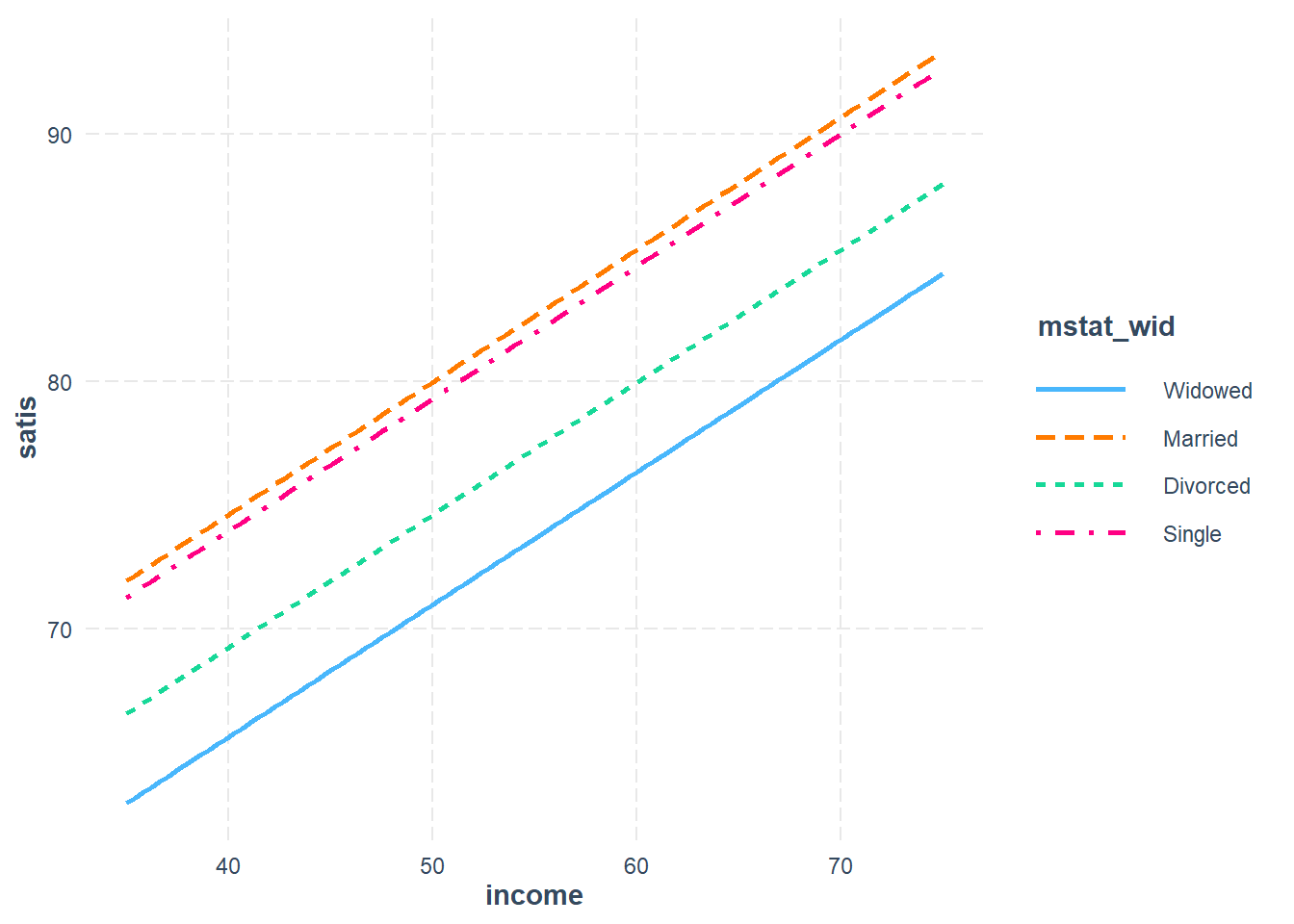 

interactions::interact_plot(model = fit_lm_3,
                            pred = income,
                            modx = mstat_wid)

interactions::interact_plot(model = fit_lm_3,
                            pred = income,
                            modx = mstat_wid,
                            legend.main = "Marital Status",
                            interval = TRUE) +
  labs(x = "Annual Income, $1000s/yr",
       y = "Estimated Marginal Mean\nLife Satisfaction") +
  theme_bw() +
  theme(legend.position = c(0, 1),
        legend.justification = c(-.1, 1.1),
        legend.key.width = unit(1.5, "cm"),
        legend.background = element_rect(color = "black"))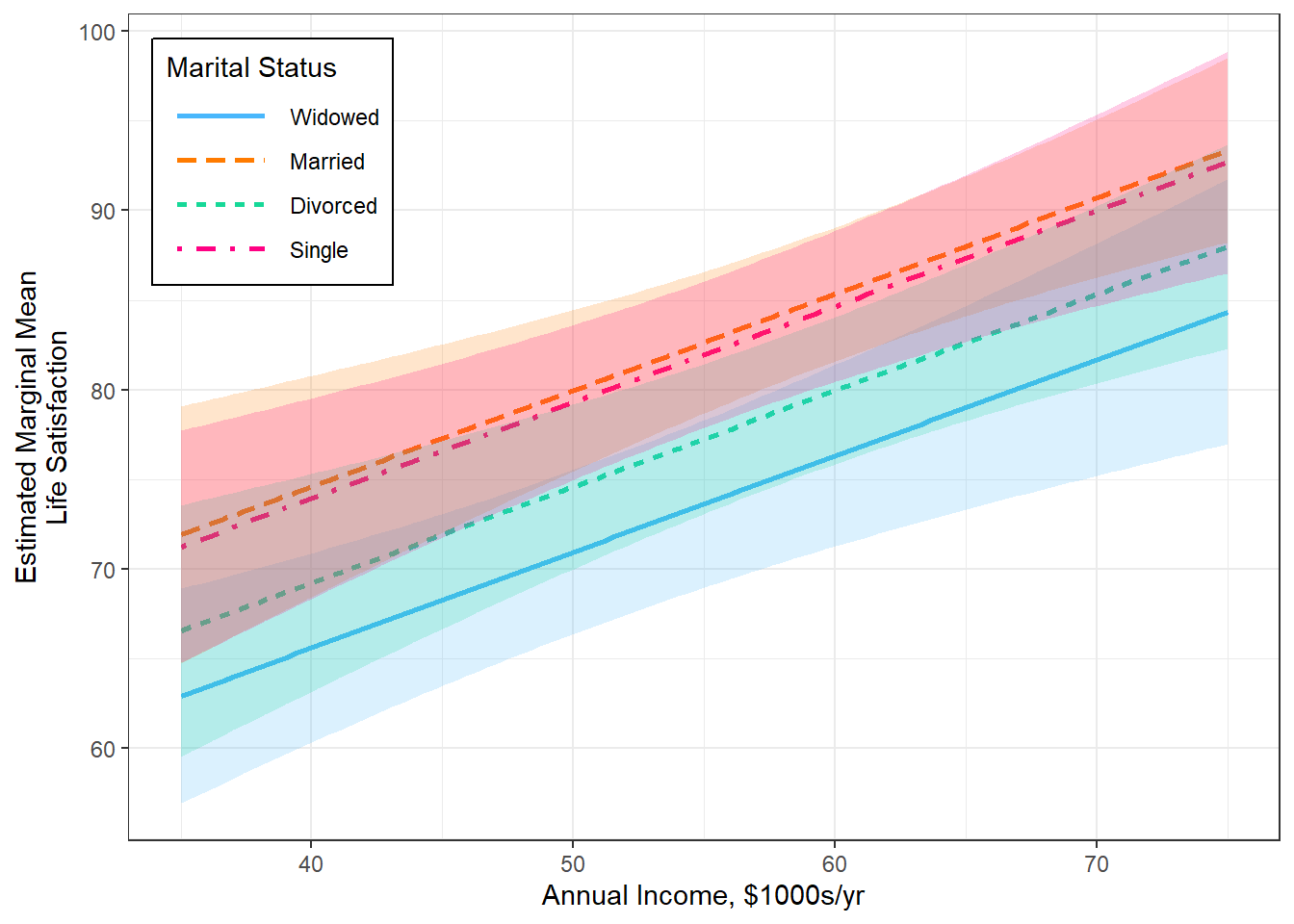

9.4.2.3 Adjust for Sex & Marital Status

Covary Sex and Marital Status

fit_lm_4 <- lm(satis ~ income + mstat_wid + sex, data = df_sat)

anova(fit_lm_4)

# A tibble: 4 × 5
     Df `Sum Sq` `Mean Sq` `F value`   `Pr(>F)`
  <int>    <dbl>     <dbl>     <dbl>      <dbl>
1     1    677.      677.     35.8    0.0000335
2     3    234.       77.9     4.12   0.0273   
3     1     11.0      11.0     0.581  0.459    
4    14    265.       18.9    NA     NA        

apaSupp::tab_lm(fit_lm_4,
                var_labels = c(income    = "Annual Income",
                               mstat_wid = "Marital Status",
                               sex       = "Male vs. Female"),
                show_single_row = "sex",
                caption = "Parameter Estimates for Life Satisfaction Regressed on Annual Income while Controlling for Marital Status and Sex",
                general_note = "Annual income is in $1000s per year.  Life Satisfaction is a composite score on a scale 1-100.") 

Table 9.11
Parameter Estimates for Life Satisfaction Regressed on Annual Income while Controlling for Marital Status and Sex

	b	(SE)	p	$b^*$	$\eta^2$	$\eta^2_p$
(Intercept)	42.20	(6.77)	< .001***
Annual Income	0.57	(0.13)	< .001***	0.68	.333	.599
Marital Status					.193	.464
Widowed	—	—
Married	10.32	(3.47)	.010*
Divorced	4.14	(3.12)	.205
Single	8.95	(3.08)	.011*
Male vs. Female	-2.02	(2.64)	.459		.009	.040
R²	.777
Adjusted R²	.697
Note. N = 20. $b^*$ = standardize coefficient; $\eta^2$ = semi-partial correlation; $\eta^2_p$ = partial correlation; p = significance from Wald t-test for parameter estimate. Annual income is in $1000s per year. Life Satisfaction is a composite score on a scale 1-100.
* p < .05. ** p < .01. *** p < .001.

apaSupp::tab_lms(list(fit_lm_2, fit_lm_3, fit_lm_4),
                 var_labels = c(mstat_wid = "Marital Status",
                                income    = "Annual Income",
                                sex       = "Sex"),
                 caption = "Comparison for Models Regressing Life Satisfaction on Annual Income, with and without Controlling for Marital Status and Sex",
                 general_note = "Annual income is in $1000s per year.  Life Satisfaction is a composite score on a scale 1-100.",
                 d = 2,
                 narrow = TRUE)

Table 9.12
Comparison for Models Regressing Life Satisfaction on Annual Income, with and without Controlling for Marital Status and Sex

	Model 1		Model 2		Model 3
Variable	b	(SE)	b	(SE)	b	(SE)
(Intercept)	44.03	(7.52) ***	44.18	(6.16) ***	42.20	(6.77) ***
Annual Income	0.64	(0.13) ***	0.54	(0.11) ***	0.57	(0.13) ***
Marital Status
Widowed			—	—	—	—
Married			9.00	(2.96) **	10.32	(3.47) *
Divorced			3.63	(3.00)	4.14	(3.12)
Single			8.33	(2.93) *	8.95	(3.08) *
Sex
Female					—	—
Male					-2.02	(2.64)
AIC	127.51		121.23		122.42
BIC	130.50		127.20		129.39
R²	.571		.768		.777
Adjusted R²	.547		.706		.697
Note. Annual income is in $1000s per year. Life Satisfaction is a composite score on a scale 1-100.
* p < .05. ** p < .01. *** p < .001.

9.5 WRITE UP

RESEARCH QUESTION:

RQ 1) Does life satisfaction differ by marital status?

RQ2) Is there an association between income and life satisfaction, after controlling for marital status?

9.5.1 Methods Section

9.5.2 Results Section

9.5.3 Table(s)

9.5.4 Figure(s)