14 Ex: Logistic - Depression (Hoffman)

Compiled: April 22, 2025

14.1 PREPARATION

14.1.1 Load Packages

# library(remotes)
# remotes::install_github("sarbearschwartz/apaSupp")  # updated: 4/15/25
# remotes::install_github("ddsjoberg/gtsummary")


library(tidyverse)
library(haven)        
library(naniar)
library(apaSupp)
library(performance) 
library(interactions)
library(GGally)

14.1.2 Load Data

This dataset comes from John Hoffman’s textbook: Regression Models for Categorical, Count, and Related Variables: An Applied Approach (2004) Amazon link, 2014 edition

Chapter 3: Logistic and Probit Regression Models

Dataset: The following example uses the SPSS data set Depress.sav. The dependent variable of interest is a measure of life satisfaction, labeled satlife.

Dependent Variable = satlife (numeric version) or lifesat (factor version)

df_depress <- haven::read_spss("https://raw.githubusercontent.com/CEHS-research/data/master/Hoffmann_datasets/depress.sav") %>% 
  haven::as_factor() %>%    # labelled to factors
  haven::zap_label() %>%    # remove SPSS junk
  haven::zap_formats() %>%  # remove SPSS junk
  haven::zap_widths() %>%   # remove SPSS junk
  dplyr::mutate(sex = forcats::fct_recode(sex,
                                          "Female" = "female",
                                          "Male" = "male")) %>% 
  dplyr::mutate(lifesat = forcats::fct_recode(lifesat,
                                              "Yes (1)" = "high",
                                              "No (0)" = "low"))

tibble::glimpse(df_depress)

Rows: 118
Columns: 14
$ id      <dbl> 1, 2, 3, 4, 5, 6, 7, 8, 9, 10, 11, 12, 13, 14, 15, 16, 17, 18,…
$ age     <dbl> 39, 41, 42, 30, 35, 44, 31, 39, 35, 33, 38, 31, 40, 44, 43, 32…
$ iq      <dbl> 94, 89, 83, 99, 94, 90, 94, 87, NA, 92, 92, 94, 91, 86, 90, NA…
$ anxiety <fct> medium low, medium low, medium high, medium low, medium low, N…
$ depress <fct> medium, medium, high, medium, low, low, medium, medium, medium…
$ sleep   <fct> low, low, low, low, high, low, NA, low, low, low, high, low, l…
$ sex     <fct> Female, Female, Female, Female, Female, Male, Female, Female, …
$ lifesat <fct> No (0), No (0), No (0), No (0), Yes (1), Yes (1), No (0), Yes …
$ weight  <dbl> 4.9, 2.2, 4.0, -2.6, -0.3, 0.9, -1.5, 3.5, -1.2, 0.8, -1.9, 5.…
$ satlife <dbl> 0, 0, 0, 0, 1, 1, 0, 1, 0, 0, 1, 1, 1, 0, 0, 1, 1, 0, 0, 1, 0,…
$ male    <dbl> 0, 0, 0, 0, 0, 1, 0, 0, 0, 0, 1, 1, 0, 0, 0, 0, 1, 0, 0, 0, 0,…
$ sleep1  <dbl> 0, 0, 0, 0, 1, 0, NA, 0, 0, 0, 1, 0, 0, 0, 0, 1, 0, 0, 0, 0, N…
$ newiq   <dbl> 2.21, -2.79, -8.79, 7.21, 2.21, -1.79, 2.21, -4.79, NA, 0.21, …
$ newage  <dbl> 1.5424, 3.5424, 4.5424, -7.4576, -2.4576, 6.5424, -6.4576, 1.5…

df_depress %>% 
  dplyr::group_by(lifesat, satlife) %>% 
  dplyr::tally()

# A tibble: 3 × 3
  lifesat satlife     n
  <fct>     <dbl> <int>
1 Yes (1)       1    52
2 No (0)        0    65
3 <NA>         NA     1

14.2 EXPLORATORY DATA ANALYSIS

14.2.1 Missing Data

df_depress %>% 
  dplyr::select("Sex" = sex,
                "Life Satisfaction" = lifesat,
                "IQ, pts" = iq,
                "Age, yrs" = age,
                "Weight, lbs" = weight) %>% 
  naniar::miss_var_summary() %>%
  dplyr::select(Variable = variable,
                n = n_miss) %>% 
  flextable::flextable() %>% 
  apaSupp::theme_apa(caption = "Missing Data by Variable")

**Table 14.1**
Missing Data by Variable
Variable	n
Weight, lbs	11
IQ, pts	8
Life Satisfaction	1
Sex	0
Age, yrs	0

df_depress %>% 
  dplyr::select("Sex" = sex,
                "Life Satisfaction" = lifesat,
                "IQ, pts" = iq,
                "Age, yrs" = age,
                "Weight, lbs" = weight) %>% 
  naniar::gg_miss_upset()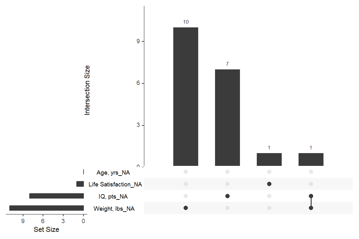

14.2.2 Summary

df_depress %>% 
  dplyr::select("Sex" = sex,
                "Life Satisfaction" = lifesat) %>% 
  apaSupp::tab_freq(caption = "Descriptive Summary of Categorical Variables")

**Table 14.2**
Descriptive Summary of Categorical Variables
		Statistic (N=118)
Sex
Male		21 (17.8%)
Female		97 (82.2%)
Life Satisfaction
Yes (1)		52 (44.1%)
No (0)		65 (55.1%)
Missing		1 (0.8%)

df_depress %>% 
  dplyr::select("IQ, pts" = iq,
                "Age, yrs" = age,
                "Weight, lbs" = weight) %>% 
  apaSupp::tab_desc(caption = "Descriptive Summary of Continuous Variables")

**Table 14.3**
Descriptive Summary of Continuous Variables
	NA	M	SD	min	Q1	Mdn	Q3	max
IQ, pts	8	91.79	4.53	82.00	89.00	92.00	94.75	106.00
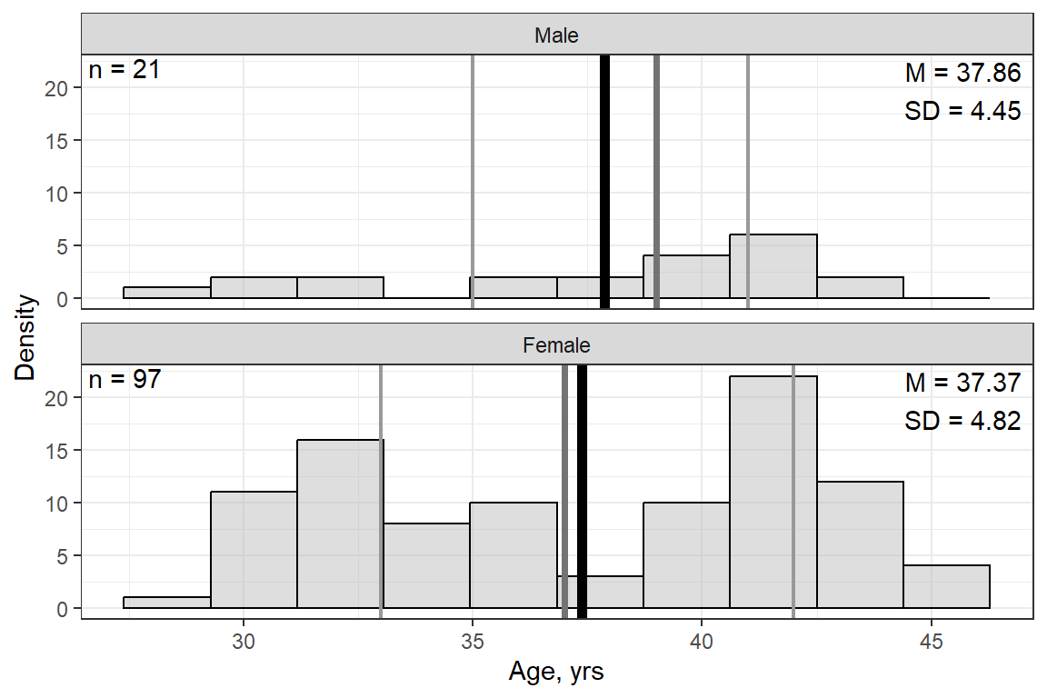
Age, yrs	0	37.46	4.74	29.00	33.00	39.00	41.75	46.00
Weight, lbs	11	1.59	2.72	-4.90	-0.65	1.70	3.55	8.30
Note. N = 118. NA = not available or missing; Mdn = median; Q1 = 25th percentile; Q3 = 75th percentile.

df_depress %>% 
  dplyr::select("Life Satisfaction" = lifesat,
                "Sex" = sex,
                "IQ" = iq,
                "Age" = age,
                "Weight" = weight) %>%
  dplyr::mutate_all(as.numeric) %>% 
  apaSupp::tab_cor(caption = "Pairwise Correlations for Life Satisfaction, Sexd, IQ, Age, and Weight") %>% 
  flextable::hline(i = 4)

**Table 14.4**
Pairwise Correlations for Life Satisfaction, Sexd, IQ, Age, and Weight
Variable Pair		r	p
Sex	Life Satisfaction	.210	.024*
IQ	Life Satisfaction	.092	.344
Age	Life Satisfaction	.100	.269
Weight	Life Satisfaction	.059	.550
IQ	Sex	.024	.806
Age	Sex	< .001	.672
Weight	Sex	.004	.968
Age	IQ	< .001	< .001***
Weight	IQ	< .001	.003**
Weight	Age	.420	< .001***
Note. N = 118. r = Pearson's Product-Moment correlation coefficient.
* p < .05. p < .01. * p < .001.

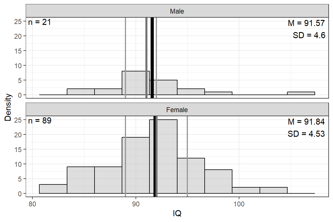
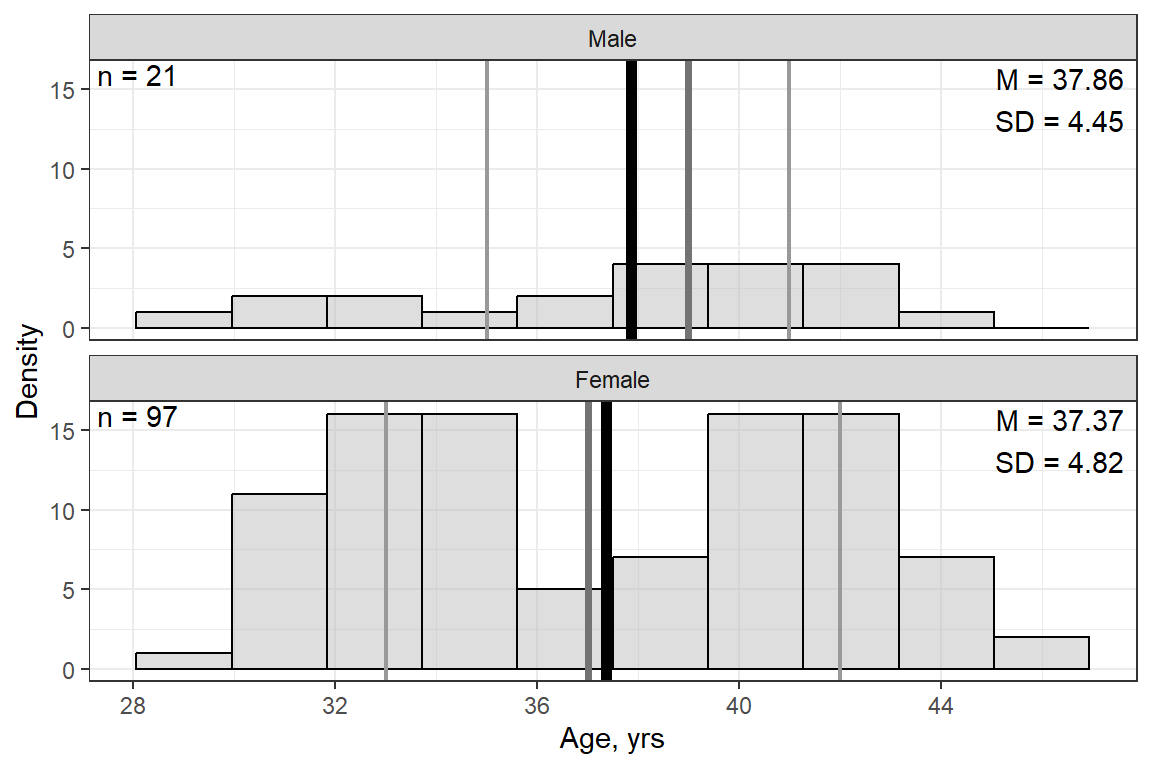
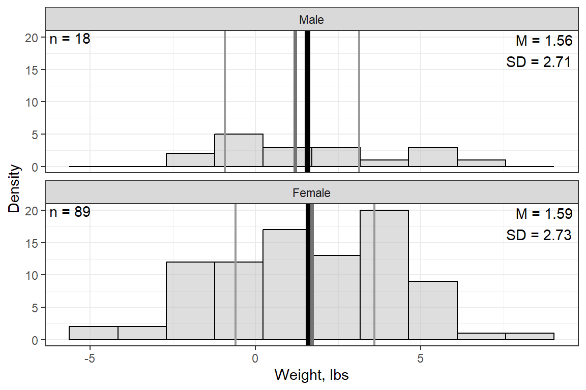
14.2.3 Visualize

df_depress %>%
  apaSupp::spicy_histos(var = iq,
                        split = sex,
                        lab = "IQ")

df_depress %>%
  apaSupp::spicy_histos(var = age,
                        split = sex,
                        lab = "Age, yrs")

df_depress %>%
  apaSupp::spicy_histos(var = weight,
                        split = sex,
                        lab = "Weight, lbs")

df_depress %>% 
  dplyr::filter(complete.cases(lifesat, sex, iq, age, weight)) %>% 
  dplyr::select("Satisfaction" = lifesat,
                "Sex" = sex,
                "IQ, pts" = iq,
                "Age, yrs" = age,
                "Weight, lbs" = weight) %>% 
  GGally::ggpairs(aes(colour = Sex),
                  diag = list(continuous = GGally::wrap("densityDiag",
                                                        alpha = .3)),
                  lower = list(continuous = GGally::wrap("smooth", 
                                                         shape = 16,
                                                         se = FALSE, 
                                                         size  = 0.75))) +
  theme_bw() +
  scale_fill_manual(values = c("blue", "coral")) +
  scale_color_manual(values = c("blue", "coral"))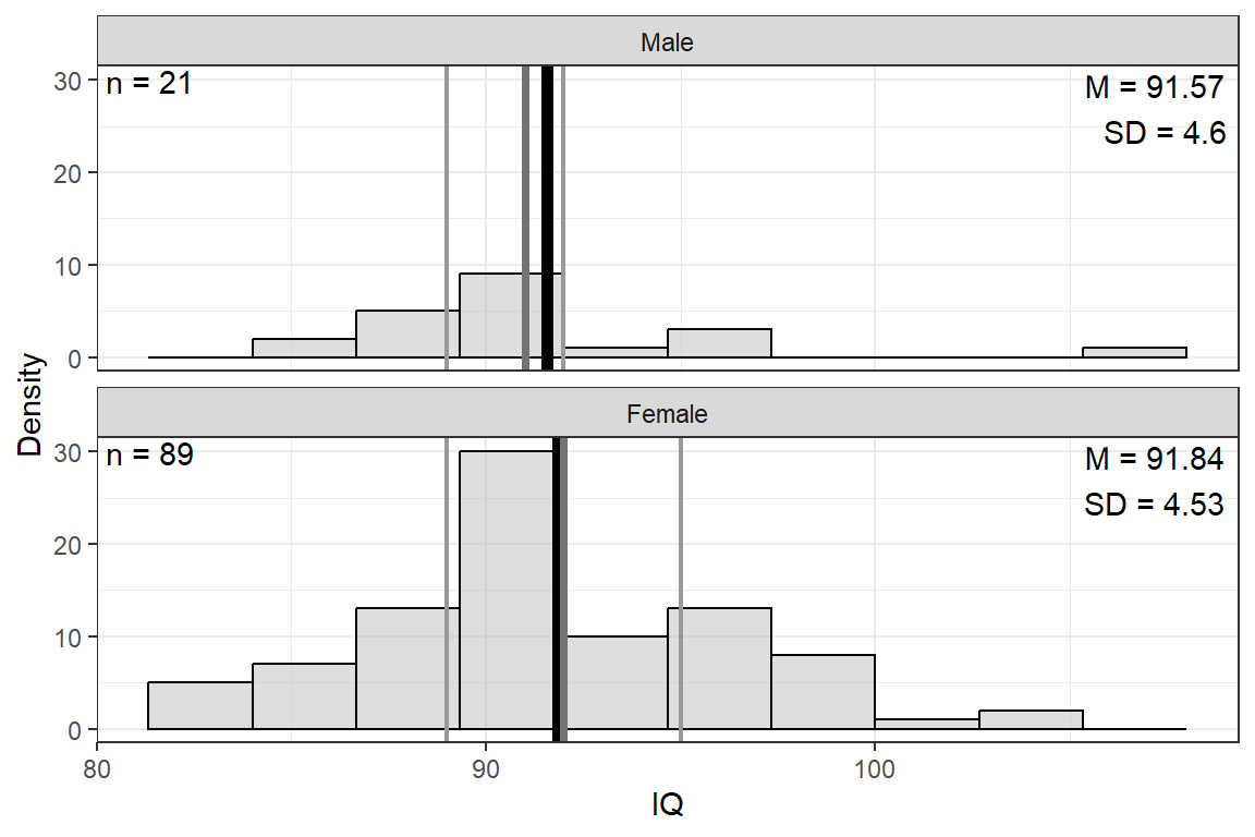

df_depress %>% 
  ggplot(aes(x = iq,
             y = satlife)) +
  geom_count() +
  geom_smooth(method = "lm") +
  theme_bw() +
  labs(x = "IQ Score",
       y = "Life Satisfaction, numeric") +
  scale_y_continuous(breaks = 0:1,
                     labels = c("No (0)", 
                                "Yes (1)"))

Figure 14.1
Hoffman’s Figure 2.3, top of page 46

df_depress %>% 
  ggplot(aes(x = weight,
             y = satlife)) +
  geom_count() +
  geom_smooth(method = "lm") +
  theme_bw() +
  labs(x = "Weight, lbs",
       y = "Life Satisfaction, numeric") +
  scale_y_continuous(breaks = 0:1,
                     labels = c("No (0)", 
                                "Yes (1)"))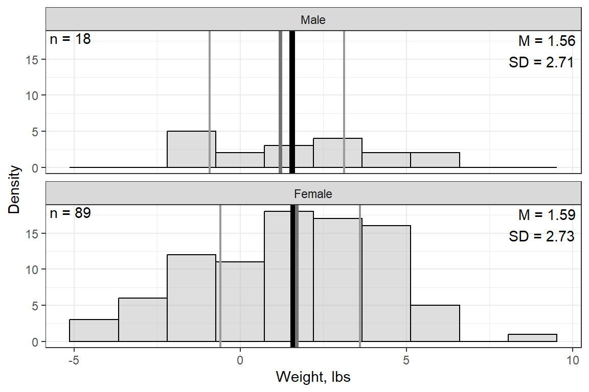

Hoffman’s Figure 2.3, top of page 46

df_depress %>% 
  ggplot(aes(x = age,
             y = satlife)) +
  geom_count() +
  geom_smooth(method = "lm") +
  theme_bw() +
  labs(x = "Age in Years",
       y = "Life Satisfaction, numeric") +
  scale_y_continuous(breaks = 0:1,
                     labels = c("No (0)", 
                                "Yes (1)"))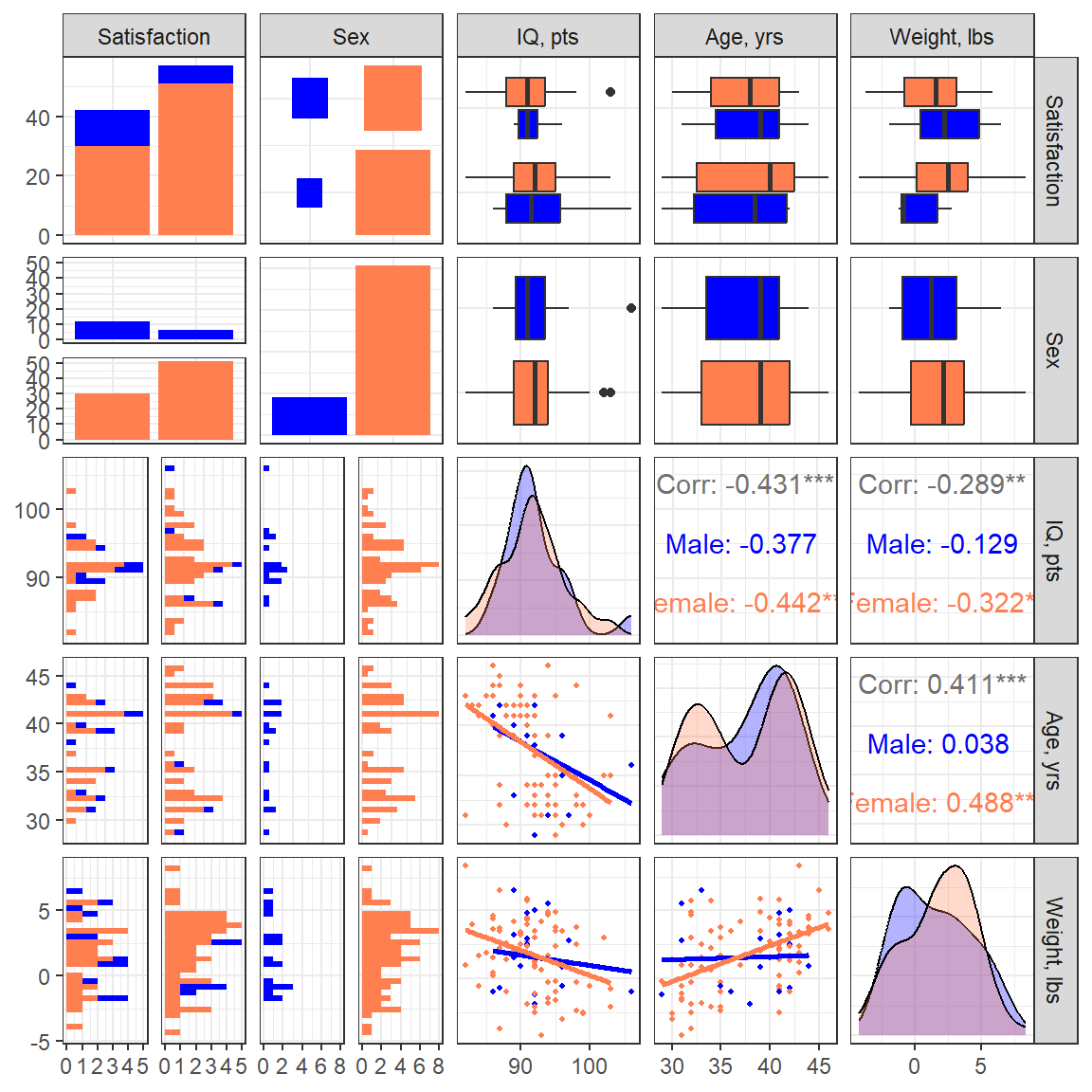

df_depress %>% 
  ggplot(aes(x = age,
             y = satlife)) +
  geom_count() +
  geom_smooth(method = "lm") +
  theme_bw() +
  labs(x = "Age in Years",
       y = "Life Satisfaction, numeric") +
  facet_grid(~ sex) +
  theme(legend.position = "none") +
  scale_y_continuous(breaks = 0:1,
                     labels = c("No (0)", 
                                "Yes (1)"))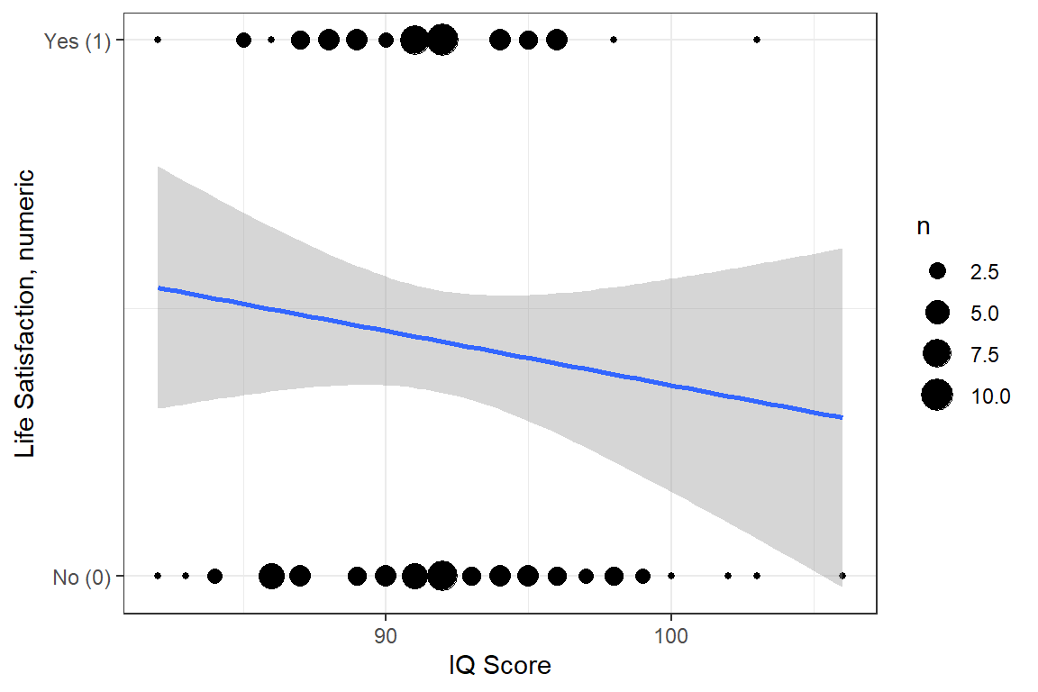

14.3 HAND CALCULATIONS

Probability, Odds, and Odds-Ratios

14.3.1 Marginal, over all the sample

Tally the number of participants who are satisfied vs. not…overall and by sex.

df_depress %>% 
  dplyr::select(sex,
                "Satisfied with Life" = lifesat) %>% 
  apaSupp::tab_freq(split = "sex",
                    caption = "Observed Life Satisfaction by Sex")

**Table 14.5**
Observed Life Satisfaction by Sex
	Male (N=21)	Female (N=97)	Total (N=118)
Satisfied with Life
Yes (1)	14 (66.7%)	38 (39.2%)	52 (44.1%)
No (0)	7 (33.3%)	58 (59.8%)	65 (55.1%)
Missing		1 (1.0%)	1 (0.8%)

14.3.1.1 Probability of being happy

\[ prob_{yes} = \frac{n_{yes}}{n_{total}} = \frac{n_{yes}}{n_{yes} + n_{no}} \]

prob <- 52 / 117

prob

[1] 0.4444444

14.3.1.2 Odds of being happy

\[ odds_{yes} = \frac{n_{yes}}{n_{no}} = \frac{n_{yes}}{n_{total} - n_{yes}} \]

odds <- 52/65

odds

[1] 0.8

\[ odds_{yes} = \frac{prob_{yes}}{prob_{no}} = \frac{prob_{yes}}{1 - prob_{yes}} \]

prob/(1 - prob)

[1] 0.8

14.3.2 Comparing by Sex

Cross-tabulate happiness (satlife) with sex (male vs. female).

df_depress %>% 
  dplyr::select(satlife, sex) %>% 
  table() %>% 
  addmargins()

       sex
satlife Male Female Sum
    0      7     58  65
    1     14     38  52
    Sum   21     96 117

14.3.2.1 Probability of being happy, by sex

Reference category = male

prob_male <- 14 / 21

prob_male

[1] 0.6666667

Comparison Category = female

prob_female <- 38 / 96

prob_female

[1] 0.3958333

14.3.2.2 Odds of being happy, by sex

Reference category = male

odds_male <- 14 / 7

odds_male

[1] 2

Comparison Category = female

odds_female <- 38 / 58


odds_female

[1] 0.6551724

14.3.2.3 Odds-Ratio for sex

\[ OR_{\text{female vs. male}} = \frac{odds_{female}}{odds_{male}} \]

odds_ratio <- odds_female / odds_male

odds_ratio

[1] 0.3275862

\[ OR_{\text{female vs. male}} = \frac{\frac{prob_{female}}{1 - prob_{female}}}{\frac{prob_{male}}{1 - prob_{male}}} \]

(prob_female / (1 - prob_female)) / (prob_male / (1 - prob_male))

[1] 0.3275862

\[ OR_{\text{female vs. male}} = \frac{\frac{n_{yes|female}}{n_{no|female}}}{\frac{n_{yes|male}}{n_{no|male}}} \]

((38 / 58)/(14 / 7))

[1] 0.3275862

14.4 SINGLE PREDICTOR

14.4.1 Fit the Model

fit_glm_1 <- glm(satlife ~ sex,
                 data = df_depress,
                 family = binomial(link = "logit"))

14.4.2 Parameter Table

apaSupp::tab_glm(fit_glm_1)

**Table 14.6**
Parameter Estimates for Generalized Linear Regression
	Odds Ratio		Logit Scale
Variable	OR	95% CI	b	(SE)	p
sex
Male	—	—	—	—
Female	0.33	[0.11, 0.86]	< .0	(0.51)	.028*
(Intercept)			0.69	(0.46)	.134
pseudo-R²	.044
Note. N = 117. CI = confidence interval. Significance denotes Wald t-tests for parameter estimates. Coefficient of deterination displays Tjur's pseudo-R².
* p < .05. p < .01. * p < .001.

apaSupp::tab_glm(fit_glm_1,
                 var_labels = c(sex = "Female vs. Male"),
                 pr2 = "both",
                 caption = "Parameter Etimates for Logistic Regressing for Life Satisfaction by Sex, Unadjusted Odds Ratio",
                 p_note = "apa1",
                 show_single_row = "sex")

**Table 14.7**
Parameter Etimates for Logistic Regressing for Life Satisfaction by Sex, Unadjusted Odds Ratio
	Odds Ratio		Logit Scale
Variable	OR	95% CI	b	(SE)	p
Female vs. Male	0.33	[0.11, 0.86]	-1.12	(0.51)	.028*
(Intercept)			0.69	(0.46)	.134
pseudo-R²
	Tjur	.044
	McFadden	.032
Note. N = 117. CI = confidence interval. Significance denotes Wald t-tests for parameter estimates. Coefficient of deterination included for both Tjur and McFadden's pseudo-R².
* p < .05.

14.4.3 Model Fit

See this commentary by Paul Alison: https://statisticalhorizons.com/r2logistic/

performance::model_performance(fit_glm_1)

# A tibble: 1 × 10
    AIC  AICc   BIC R2_Tjur  RMSE Sigma Log_loss Score_log Score_spherical   PCP
  <dbl> <dbl> <dbl>   <dbl> <dbl> <dbl>    <dbl>     <dbl>           <dbl> <dbl>
1  160.  160.  165.  0.0437 0.486     1    0.665     -30.1          0.0550 0.528

performance::r2(fit_glm_1)

# R2 for Logistic Regression
  Tjur's R2: 0.044

performance::r2_mcfadden(fit_glm_1)

# R2 for Generalized Linear Regression
       R2: 0.032
  adj. R2: 0.019

14.4.4 Predicted Probability

14.4.4.1 Logit scale

fit_glm_1 %>% 
  emmeans::emmeans(~ sex)

 sex    emmean    SE  df asymp.LCL asymp.UCL
 Male    0.693 0.463 Inf    -0.214    1.6004
 Female -0.423 0.209 Inf    -0.832   -0.0138

Results are given on the logit (not the response) scale. 
Confidence level used: 0.95

fit_glm_1 %>% 
  emmeans::emmeans(~ sex) %>% 
  pairs()

 contrast      estimate    SE  df z.ratio p.value
 Male - Female     1.12 0.508 Inf   2.198  0.0280

Results are given on the log odds ratio (not the response) scale.

14.4.4.2 Response Scale

Probability

fit_glm_1 %>% 
  emmeans::emmeans(~ sex,
                   type = "response")

 sex     prob     SE  df asymp.LCL asymp.UCL
 Male   0.667 0.1030 Inf     0.447     0.832
 Female 0.396 0.0499 Inf     0.303     0.497

Confidence level used: 0.95 
Intervals are back-transformed from the logit scale

fit_glm_1 %>% 
  emmeans::emmeans(~ sex,
                   type = "response") %>% 
  pairs()

 contrast      odds.ratio   SE  df null z.ratio p.value
 Male / Female       3.05 1.55 Inf    1   2.198  0.0280

Tests are performed on the log odds ratio scale

14.4.5 Interpretation

On average, two out of every three males is satisfied, b = 0.667, odds = 1.95, 95% CI [1.58, 2.40].
Females have 67% lower odds of being depressed, compared to men, b = -0.27, OR = 0.77, 95% CI [0.61, 0.96], p = .028.

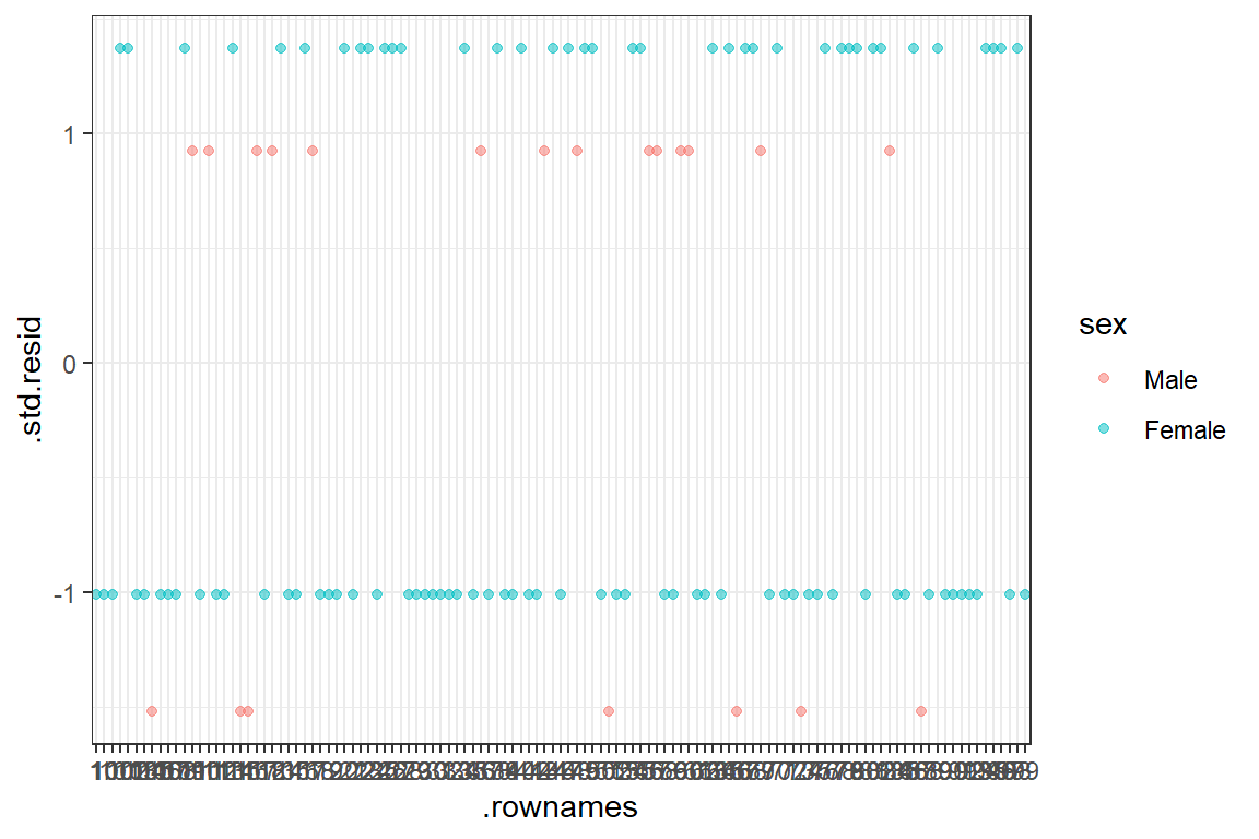
14.4.6 Diagnostics

14.4.6.1 Influential values

Influential values are extreme individual data points that can alter the quality of the logistic regression model.

The most extreme values in the data can be examined by visualizing the Cook’s distance values. Here we label the top 7 largest values:

plot(fit_glm_1, which = 4, id.n = 7)

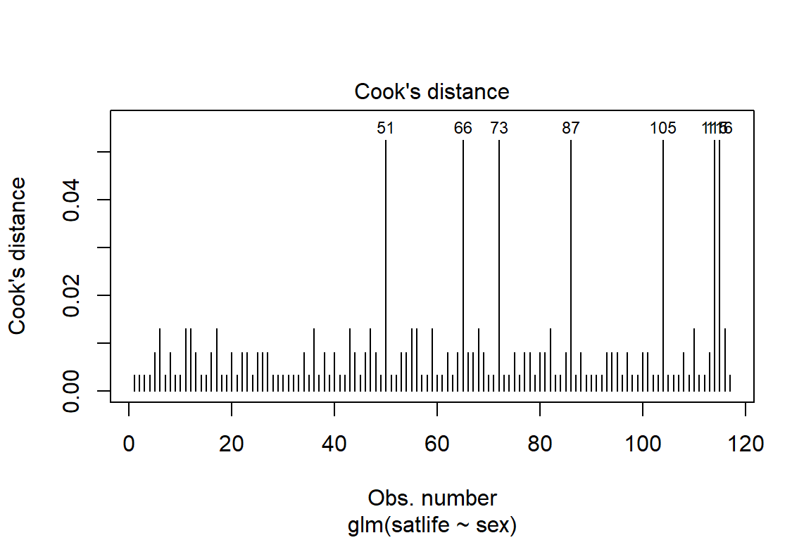
Note that, not all outliers are influential observations. To check whether the data contains potential influential observations, the standardized residual error can be inspected. Data points with an absolute standardized residuals above 3 represent possible outliers and may deserve closer attention.

14.4.6.2 Standardized Residuals

The following R code computes the standardized residuals (.std.resid) using the R function augment() [broom package].

fit_glm_1 %>% 
  broom::augment() %>% 
  ggplot(aes(x = .rownames, .std.resid)) + 
  geom_point(aes(color = sex), alpha = .5) +
  theme_bw()

14.5 MULTIPLE PREDICTORS

14.5.1 Fit the Model

fit_glm_2 <- glm(satlife ~ sex + iq + age + weight,
                 data = df_depress,
                 family = binomial(link = "logit"))

14.5.2 Parameter Table

EXAMPLE 3.3 A Logistic Regression Model of Life Satisfaction with Multiple Independent Variables, middle of page 52

apaSupp::tab_glm(fit_glm_2)

**Table 14.8**
Parameter Estimates for Generalized Linear Regression
	Odds Ratio		Logit Scale
Variable	OR	95% CI	b	(SE)	Wald	LRT	VIF
sex						.018*	1.01
Male	—	—	—	—
Female	0.28	[0.09, 0.81]	< .0	(0.56)	.022*
iq	0.93	[0.83, 1.03]	-0.07	(0.05)	.174	.167	1.29
age	0.96	[0.86, 1.06]	-0.04	(0.05)	.433	.431	1.42
weight	0.96	[0.81, 1.15]	-0.04	(0.09)	.671	.671	1.23
(Intercept)			9.02	(6.02)	.134
pseudo-R²	.075
Note. N = 99. CI = confidence interval; VIF = variance inflation factor. Significance denotes Wald t-tests for individual parameter estimates, as well as Likelihood Ratio Tests (LRT) for single-predictor deletion. Coefficient of deterination displays Tjur's pseudo-R².
* p < .05. p < .01. * p < .001.

apaSupp::tab_glm(fit_glm_2, vif = FALSE, pr2 = "both")

**Table 14.9**
Parameter Estimates for Generalized Linear Regression
	Odds Ratio		Logit Scale
Variable	OR	95% CI	b	(SE)	Wald	LRT
sex						.018*
Male	—	—	—	—
Female	0.28	[0.09, 0.81]	< .0	(0.56)	.022*
iq	0.93	[0.83, 1.03]	-0.07	(0.05)	.174	.167
age	0.96	[0.86, 1.06]	-0.04	(0.05)	.433	.431
weight	0.96	[0.81, 1.15]	-0.04	(0.09)	.671	.671
(Intercept)			9.02	(6.02)	.134
pseudo-R²
	Tjur	.075
	McFadden	.207
Note. N = 99. CI = confidence interval. Significance denotes Wald t-tests for individual parameter estimates, as well as Likelihood Ratio Tests (LRT) for single-predictor deletion. Coefficient of deterination included for both Tjur and McFadden's pseudo-R².
* p < .05. p < .01. * p < .001.

apaSupp::tab_glm(fit_glm_2, fit = c("AIC", "BIC"))

**Table 14.10**
Parameter Estimates for Generalized Linear Regression
	Odds Ratio		Logit Scale
Variable	OR	95% CI	b	(SE)	Wald	LRT	VIF
sex						.018*	1.01
Male	—	—	—	—
Female	0.28	[0.09, 0.81]	< .0	(0.56)	.022*
iq	0.93	[0.83, 1.03]	-0.07	(0.05)	.174	.167	1.29
age	0.96	[0.86, 1.06]	-0.04	(0.05)	.433	.431	1.42
weight	0.96	[0.81, 1.15]	-0.04	(0.09)	.671	.671	1.23
AIC	138
BIC	150
(Intercept)			9.02	(6.02)	.134
pseudo-R²	.075
Note. N = 99. CI = confidence interval; VIF = variance inflation factor. Significance denotes Wald t-tests for individual parameter estimates, as well as Likelihood Ratio Tests (LRT) for single-predictor deletion. Coefficient of deterination displays Tjur's pseudo-R².
* p < .05. p < .01. * p < .001.

apaSupp::tab_glm(fit_glm_2, vif = FALSE, lrt = FALSE)

**Table 14.11**
Parameter Estimates for Generalized Linear Regression
	Odds Ratio		Logit Scale
Variable	OR	95% CI	b	(SE)	p
sex
Male	—	—	—	—
Female	0.28	[0.09, 0.81]	< .0	(0.56)	.022*
iq	0.93	[0.83, 1.03]	-0.07	(0.05)	.174
age	0.96	[0.86, 1.06]	-0.04	(0.05)	.433
weight	0.96	[0.81, 1.15]	-0.04	(0.09)	.671
(Intercept)			9.02	(6.02)	.134
pseudo-R²	.075
Note. N = 99. CI = confidence interval. Significance denotes Wald t-tests for parameter estimates. Coefficient of deterination displays Tjur's pseudo-R².
* p < .05. p < .01. * p < .001.

apaSupp::tab_glm(fit_glm_2,
                 var_labels = c(sex = "Female vs. Male",
                                iq = "IQ, pts",
                                age = "Age, yrs",
                                weight = "Weight, lbs"), 
                 pr2 = "both",
                 show_single_row = "sex",
                 p_note = "apa1",
                 caption = "Parameter Etimates for Logistic Regressing for Life Satisfaction by Sex, Controlling fro IQ, Age, and Weight") %>% 
  flextable::bold(i = c(2))

**Table 14.12**
Parameter Etimates for Logistic Regressing for Life Satisfaction by Sex, Controlling fro IQ, Age, and Weight
	Odds Ratio		Logit Scale
Variable	OR	95% CI	b	(SE)	Wald	LRT	VIF
Female vs. Male	0.28	[0.09, 0.81]	-1.28	(0.56)	.022*	.018*	1.01
IQ, pts	0.93	[0.83, 1.03]	-0.07	(0.05)	.174	.167	1.29
Age, yrs	0.96	[0.86, 1.06]	-0.04	(0.05)	.433	.431	1.42
Weight, lbs	0.96	[0.81, 1.15]	-0.04	(0.09)	.671	.671	1.23
(Intercept)			9.02	(6.02)	.134
pseudo-R²
	Tjur	.075
	McFadden	.207
Note. N = 99. CI = confidence interval; VIF = variance inflation factor. Significance denotes Wald t-tests for individual parameter estimates, as well as Likelihood Ratio Tests (LRT) for single-predictor deletion. Coefficient of deterination included for both Tjur and McFadden's pseudo-R².
* p < .05.

apaSupp::tab_glm_fits(list("Univariate"   = fit_glm_1, 
                           "Multivariate" = fit_glm_2))

**Table 14.13**
Comparison of Generalized Linear Model Performane Metrics
			pseudo- $R^2$
Model	N	k	McFadden	Tjur	AIC	BIC	RMSE
Univariate	117	2	.032	.044	159.62	165.14	0.49
Multivariate	99	5	.207	.075	137.52	150.50	0.47
Note. Models fit to different samples. k = number of parameters estimated in each model. Larger $R^2$ values indicated better performance. Smaller values indicated better performance for Akaike's Information Criteria (AIC), Bayesian information criteria (BIC), and Root Mean Squared Error (RMSE).

14.6 COMPARE MODELS

14.6.1 Refit to Complete Cases

Restrict the data to only participant that have all four of these predictors.

df_depress_model <- df_depress %>% 
  dplyr::filter(complete.cases(satlife, 
                               sex, iq, age, weight))

Refit Model 1 with only participant complete on all the predictors.

fit_glm_1_redo <- glm(satlife ~ sex,
                      data = df_depress_model,
                      family = binomial(link = "logit"))

fit_glm_2_redo <- glm(satlife ~ sex + iq + age + weight,
                      data = df_depress_model,
                      family = binomial(link = "logit"))

14.6.2 Parameter Table

apaSupp::tab_glms(list(fit_glm_1_redo, fit_glm_2_redo))

**Table 14.14**
Compare Generalized Regression Models
	Model 1			Model 2
Variable	OR	95% CI	p	OR	95% CI	p
sex
Male	—	—		—	—
Female	0.29	[0.09, 0.84]	.026*	0.28	[0.09, 0.81]	.022*
iq				0.93	[0.83, 1.03]	.174
age				0.96	[0.86, 1.06]	.433
weight				0.96	[0.81, 1.15]	.671
Fit Metrics
AIC	133.7			137.5
BIC	138.9			150.5
pseudo-R²
Tjur	.053			.075
McFadden	.039			.055
Note. N = 99. CI = confidence interval.Coefficient of deterination estiamted with both Tjur and McFadden's psuedo R-squared
* p < .05. p < .01. * p < .001.

apaSupp::tab_glms(list("Univariate"   = fit_glm_1_redo, 
                       "Multivariate" = fit_glm_2_redo),
                  var_labels = c(sex = "Sex",
                                 iq = "IQ Score",
                                 age = "Age, yrs",
                                 weight = "Weight, lbs"),
                  fit = "AIC",
                  pr2 = "tjur",
                  narrow = TRUE) %>% 
  flextable::bold(i = 3)

**Table 14.15**
Compare Generalized Regression Models
	Univariate		Multivariate
Variable	OR	95% CI	OR	95% CI
Sex
Male	—	—	—	—
Female	0.29	[0.09, 0.84]*	0.28	[0.09, 0.81]*
IQ Score			0.93	[0.83, 1.03]
Age, yrs			0.96	[0.86, 1.06]
Weight, lbs			0.96	[0.81, 1.15]
AIC	133.70		137.52
pseudo-R²	.053		.075
Note. N = 99. CI = confidence interval.Coefficient of deterination estiamted by Tjur's psuedo R-squared
* p < .05. p < .01. * p < .001.

14.6.3 Comparison Criteria

apaSupp::tab_glm_fits(list("Univariate, Initial"   = fit_glm_1, 
                           "Univariate, Restricted" = fit_glm_1_redo, 
                           "Multivariate" = fit_glm_2_redo))

**Table 14.16**
Comparison of Generalized Linear Model Performane Metrics
			pseudo- $R^2$
Model	N	k	McFadden	Tjur	AIC	BIC	RMSE
Univariate, Initial	117	2	.032	.044	159.62	165.14	0.49
Univariate, Restricted	99	2	.039	.053	133.70	138.89	0.48
Multivariate	99	5	.055	.075	137.52	150.50	0.47
Note. Models fit to different samples. k = number of parameters estimated in each model. Larger $R^2$ values indicated better performance. Smaller values indicated better performance for Akaike's Information Criteria (AIC), Bayesian information criteria (BIC), and Root Mean Squared Error (RMSE).

anova(fit_glm_1_redo, 
      fit_glm_2_redo,
      test = "LRT")

# A tibble: 2 × 5
  `Resid. Df` `Resid. Dev`    Df Deviance `Pr(>Chi)`
        <dbl>        <dbl> <dbl>    <dbl>      <dbl>
1          97         130.    NA    NA        NA    
2          94         128.     3     2.18      0.537

14.6.4 Interpretation

Only sex is predictive of depression. There is no evidence IQ, age, or weight are associated with depression, LRT $\chi^2$(3) = 2.17, p = .537.

14.7 CHANGING REFERENCE CATEGORY

levels(df_depress$sex)

[1] "Male"   "Female"

df_depress_ref <- df_depress %>% 
  dplyr::mutate(male   = sex %>% forcats::fct_relevel("Female", after = 0)) %>%   dplyr::mutate(female = sex %>% forcats::fct_relevel("Male",   after = 0))

levels(df_depress_ref$male)

[1] "Female" "Male"

levels(df_depress_ref$female)

[1] "Male"   "Female"

fit_glm_2_male <- glm(satlife ~ male + iq + age + weight,
                      data = df_depress_ref,
                      family = binomial(link = "logit"))

fit_glm_2_female <- glm(satlife ~ female + iq + age + weight,
                        data = df_depress_ref,
                        family = binomial(link = "logit"))

apaSupp::tab_glms(list("Reference = Male"  = fit_glm_2_female,
                       "Reference = Female" = fit_glm_2_male)) %>% 
  flextable::bold(i = c(3, 9))

**Table 14.17**
Compare Generalized Regression Models
	Reference = Male			Reference = Female
Variable	OR	95% CI	p	OR	95% CI	p
female
Male	—	—
Female	0.28	[0.09, 0.81]	.022*
iq	0.93	[0.83, 1.03]	.174	0.93	[0.83, 1.03]	.174
age	0.96	[0.86, 1.06]	.433	0.96	[0.86, 1.06]	.433
weight	0.96	[0.81, 1.15]	.671	0.96	[0.81, 1.15]	.671
male
Female				—	—
Male				3.59	[1.24, 11.49]	.022*
Fit Metrics
AIC	137.5			137.5
BIC	150.5			150.5
pseudo-R²
Tjur	.075			.075
McFadden	.207			.207
Note. N = 99. CI = confidence interval.Coefficient of deterination estiamted with both Tjur and McFadden's psuedo R-squared
* p < .05. p < .01. * p < .001.