13 Ex: Ihno’s Experiment

interaction between two continuous IVs

# library(remotes)
# remotes::install_github("sarbearschwartz/apaSupp")
# remotes::install_github("ddsjoberg/gtsummary")

library(tidyverse)       
library(haven)   
library(naniar)       
library(apaSupp)
library(corrplot)
library(GGally)
library(performance)
library(interactions)
library(ggResidpanel)
library(car)

13.1 PURPOSE

13.1.1 Research Question

Does math phobia moderate the relationship between math and statistics performance? That is, does the assocation between math and stat quiz performance differ at variaous levels of math phobia?

13.1.2 Data Description

Inho’s dataset is included in the textbook “Explaining Psychological Statistics” (Cohen 2013) and details regarding the sample and measures is describe in this Encyclopedia’s Vol. 2 - Ihno’s Dataset.

13.1.2.1 Variables

statquiz dependent variable (DV, Y): stat quiz score, max = 10
mathquiz independent variable (IC, X1): prior math quiz score, max = 50
phobia independent variable (IC, X2): self-reported math phobia, score of 0-10

df_ihno <- haven::read_spss("https://raw.githubusercontent.com/CEHS-research/eBook_regression/master/data/Ihno_dataset.sav") %>% 
  haven::zap_widths() %>% 
  haven::zap_label() %>% 
  haven::zap_formats() %>% 
  dplyr::rename_all(tolower) %>% 
  dplyr::mutate(gender = factor(gender, 
                                levels = c(1, 2),
                                labels = c("Female", 
                                           "Male"))) %>% 
  dplyr::mutate(major = factor(major, 
                               levels = c(1, 2, 3, 4,5),
                               labels = c("Psychology",
                                          "Premed",
                                          "Biology",
                                          "Sociology",
                                          "Economics"))) %>% 
  dplyr::mutate(reason = factor(reason,
                                levels = c(1, 2, 3),
                                labels = c("Program requirement",
                                           "Personal interest",
                                           "Advisor recommendation"))) %>% 
  dplyr::mutate(exp_cond = factor(exp_cond,
                                  levels = c(1, 2, 3, 4),
                                  labels = c("Easy",
                                             "Moderate",
                                             "Difficult",
                                             "Impossible"))) %>% 
  dplyr::mutate(coffee = factor(coffee,
                                levels = c(0, 1),
                                labels = c("Not a regular coffee drinker",
                                           "Regularly drinks coffee"))) %>% 
  dplyr::mutate(mathquiz = as.numeric(mathquiz))

df_ihno %>% 
  dplyr::select(phobia, mathquiz, statquiz) %>% 
  tibble::glimpse()

Rows: 100
Columns: 3
$ phobia   <dbl> 1, 1, 4, 4, 10, 4, 4, 4, 4, 5, 5, 4, 7, 4, 3, 8, 4, 5, 0, 4, …
$ mathquiz <dbl> 43, 49, 26, 29, 31, 20, 13, 23, 38, NA, 29, 32, 18, NA, 21, N…
$ statquiz <dbl> 6, 9, 8, 7, 6, 7, 3, 7, 8, 7, 8, 8, 1, 5, 8, 3, 8, 7, 10, 7, …

13.2 EXPLORATORY DATA ANALYSIS

Before embarking on any inferential analysis or modeling, always get familiar with your variables one at a time (univariate), as well as pairwise (bivariate).

13.2.1 Summary Statistics

13.2.1.1 Univariate

Center: mean and median Spread: standard deviation, range (max - min), interquartile range (Q3 - Q1)

df_ihno %>% 
  dplyr::select("Math Phobia" = phobia,
                "Math Quiz" = mathquiz,
                "Stat Quiz" = statquiz) %>% 
  apaSupp::tab_desc(caption = "Descriptive Summary of Participants")

**Table 13.1**
Descriptive Summary of Participants
Variable	NA	M	SD	min	Q1	Mdn	Q3	max
Math Phobia	0	3.31	2.44	0.00	1.00	3.00	4.00	10.00
Math Quiz	15	29.07	9.48	9.00	22.00	30.00	35.00	49.00
Stat Quiz	0	6.86	1.70	1.00	6.00	7.00	8.00	10.00
Note. NA = not available or missing. Mdn = median. Q1 = 25th percentile, Q3 = 75th percentile. N = 100.

13.2.1.2 Bivariate

When two variables are both continuous, correlations (Pearson’s \(R\)) are an important measure of association.

Notice the discrepancy between the correlation between statquiz and phobia. Above, the psych::pairs.panels() function uses pairwise complete cases by default, so \(r=-.39\) is computed on all \(n=100\) subjects. Below, we specified use = "complete.obs" in the cor() function, so all correlations will be based on the same \(n=85\) students, making it list wise complete. The choice of which method to you will vary by situation.

Often it is easier to digest a correlation matrix if it is visually presented, instead of just given as a table of many numbers. The corrplot package has a useful function called corrplot.mixed() for doing just that (Wei and Simko 2024).

df_ihno %>% 
  dplyr::select(phobia, mathquiz, statquiz) %>% 
  cor(use = "complete.obs") %>% 
  corrplot::corrplot.mixed(lower  = "ellipse",
                           upper  = "number",
                           tl.col = "black")

Figure 13.1
Visualize Correlation Matrix

df_ihno %>% 
  dplyr::select("Math Phobia" = phobia,
                "Math Quiz" = mathquiz,
                "Stat Quiz" = statquiz) %>% 
  apaSupp::tab_cor(caption = "Correlations")

**Table 13.2**
Correlations
Variables		r	p
Math Phobia	Math Quiz	-0.280	.009	**
Math Phobia	Stat Quiz	-0.390	< .001	***
Math Quiz	Stat Quiz	0.510	< .001	***
Note. r = Pearson's Product-Moment correlation coefficient. N = 100.
* p < .05. p < .01. * p < .001.

13.2.2 Visualize Distributions

13.2.2.1 Univariate

Always plot your data first!

df_ihno %>% 
  apaSupp::spicy_histos(var = phobia)

Figure 13.2
Distribution of Self-Reported Math Phobia

df_ihno %>% 
  apaSupp::spicy_histos(var = mathquiz)

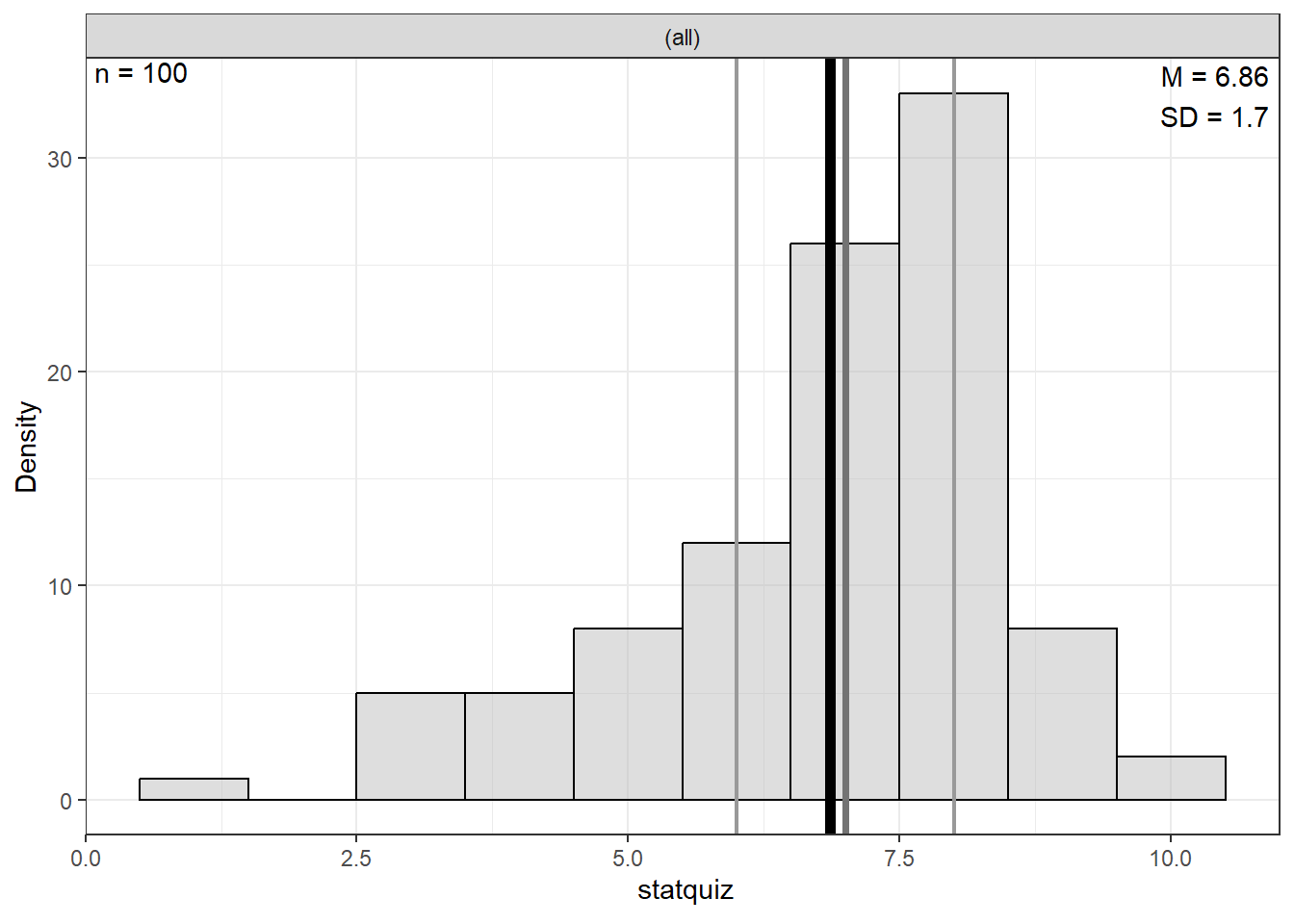
Figure 13.3
Distribution of Prior Math Quiz Performance

df_ihno %>% 
  apaSupp::spicy_histos(var = statquiz)

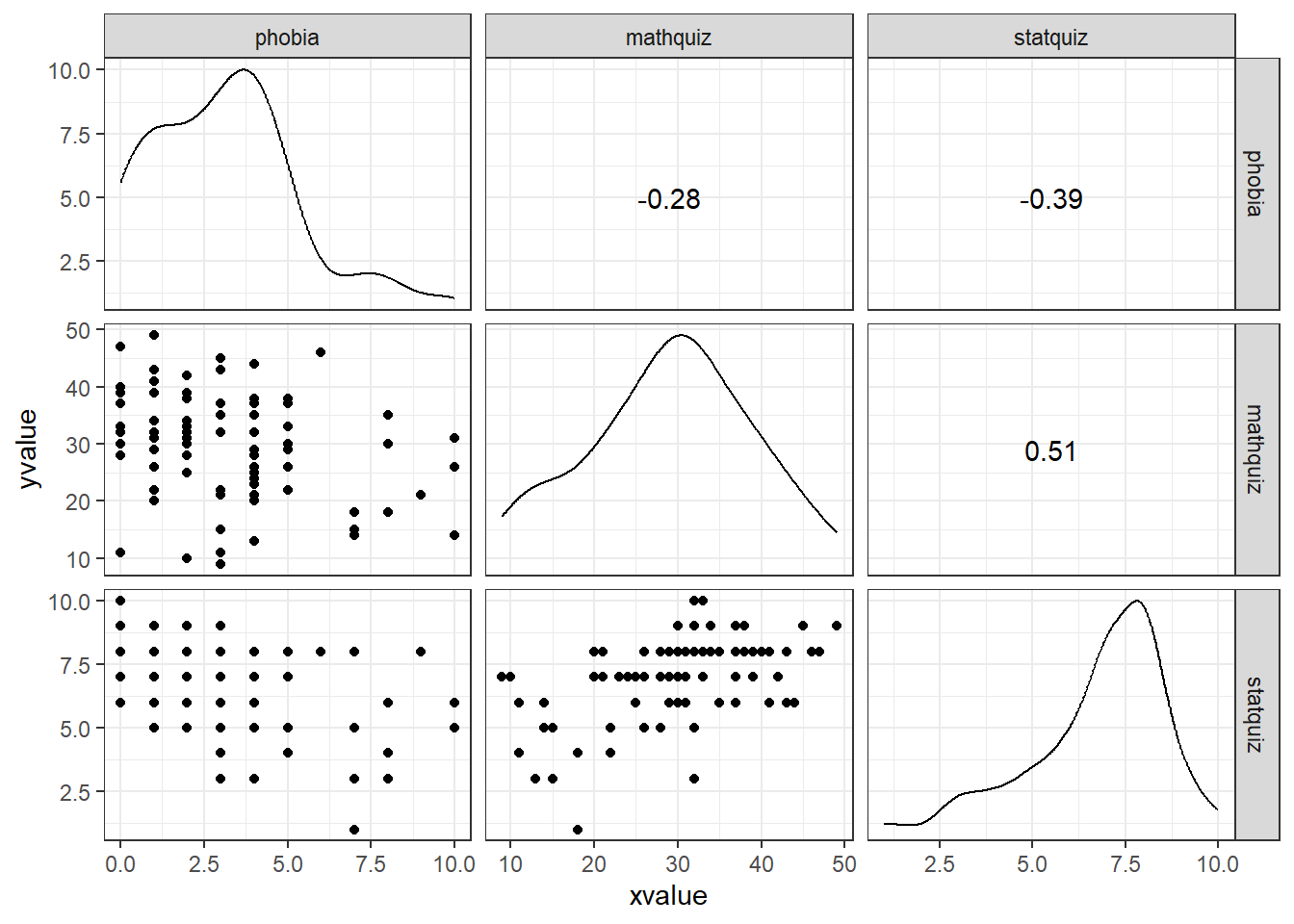
Figure 13.4
Distribution of Statistics Quiz Performance

13.2.2.2 Bivariate

df_ihno %>% 
  dplyr::select(phobia, mathquiz, statquiz) %>% 
  data.frame %>% 
  GGally::ggscatmat() +
  theme_bw()

Figure 13.5
Pairs Plot

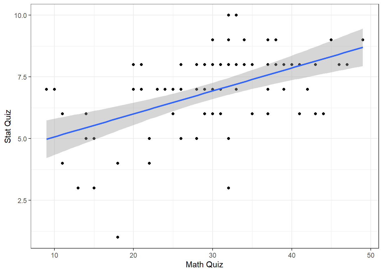
df_ihno %>% 
  ggplot(aes(x = mathquiz,
             y = statquiz)) +
  geom_point() +
  theme_bw() +
  geom_smooth(method = "lm",
              formula = y ~ x) +
  labs(x = "Math Quiz",
       y = "Stat Quiz")

Figure 13.6
Scatterplot for Stat Quiz Regressed on Math Quiz

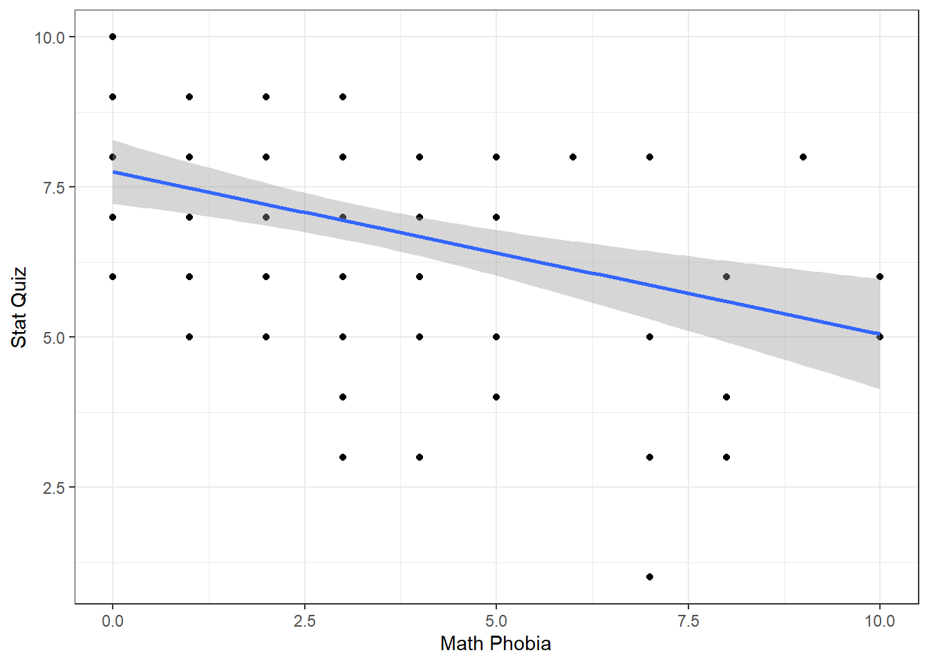
df_ihno %>% 
  ggplot(aes(x = phobia,
             y = statquiz)) +
  geom_point() +
  theme_bw() +
  geom_smooth(method = "lm",
              formula = y ~ x) +
  labs(x = "Math Phobia",
       y = "Stat Quiz")

Figure 13.7
Scatterplot for Stat Quiz Regressed on Phobia

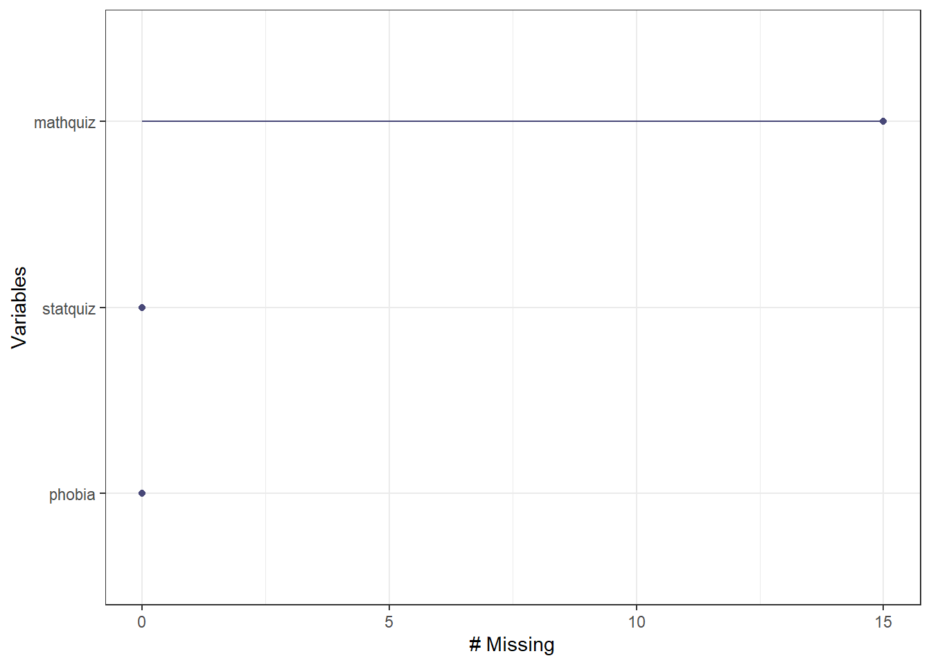
13.2.3 Missing Values

It turns out that 15 of the 100 students did not have a math quiz score recorded.

df_ihno %>%
  dplyr::select(mathquiz, statquiz, phobia) %>% 
  naniar::gg_miss_var() +
  theme_bw()

Figure 13.8
Missingness on Each Variable

df_ihno %>% 
  dplyr::filter(!complete.cases(mathquiz, statquiz, phobia)) %>% 
  dplyr::select(sub_num, mathquiz, statquiz, phobia)

# A tibble: 15 × 4
   sub_num mathquiz statquiz phobia
     <dbl>    <dbl>    <dbl>  <dbl>
 1      10       NA        7      5
 2      14       NA        5      4
 3      16       NA        3      8
 4      20       NA        7      4
 5      29       NA        7      3
 6      32       NA        7      3
 7      42       NA        9      0
 8      49       NA        5      5
 9      51       NA        7      4
10      57       NA        8      2
11      65       NA        8      5
12      70       NA        7      3
13      77       NA        8      1
14      88       NA        8      1
15      95       NA        8      7

13.3 REGRESSION ANALYSIS

The lm() function must be supplied with at least two options:

a formula: Y ~ X
a dataset: data = XXXXXXX

When a model is fit and directly saved as a named object via the assignment opperator (<-), no output is produced.

The dependent variable (DV) is Stat Quiz score, statquiz (\(Y\))
The independent variables (IVs) are both math quiz score mathquiz and math phobia phobia(\(X_1\), \(X_2\))

All regression models can only be fit to complete observations regarding the variables included in the model (dependent and independent). Removing any case that is incomplete with respect to even one variables is called “list-wise deletion”.

In this analysis, models including the mathquiz variable will be fit on only 85 students (since 15 students did not take the math quiz), where as models not including this variable will be fit to all 100 students.

This complicates model comparisons, which require nested models be fit to the same data (exactly). For this reason, the dataset has been reduced to the subset of students that are complete regarding the three variables utilized throughout the set of five nested models.

df_ihno_fitting <- df_ihno %>% 
  dplyr::select(mathquiz, statquiz, phobia) %>% 
  dplyr::filter(complete.cases(mathquiz, statquiz, phobia))

tibble::glimpse(df_ihno_fitting)

Rows: 85
Columns: 3
$ mathquiz <dbl> 43, 49, 26, 29, 31, 20, 13, 23, 38, 29, 32, 18, 21, 37, 37, 3…
$ statquiz <dbl> 6, 9, 8, 7, 6, 7, 3, 7, 8, 8, 8, 1, 8, 8, 7, 10, 7, 4, 8, 8, …
$ phobia   <dbl> 1, 1, 4, 4, 10, 4, 4, 4, 4, 5, 4, 7, 3, 4, 5, 0, 4, 3, 4, 0, …

13.3.1 Fit Models

The bottom-up approach consists of starting with an initial NULL model with only an intercept term and them building additional models that are nested.

Two models are considered nested if one is contains a subset of the terms (predictors or IV) compared to the other.

fit_ihno_lm_0 <- lm(statquiz ~ 1,                 data = df_ihno_fitting)
fit_ihno_lm_1 <- lm(statquiz ~ mathquiz,          data = df_ihno_fitting)
fit_ihno_lm_2 <- lm(statquiz ~ phobia,            data = df_ihno_fitting)
fit_ihno_lm_3 <- lm(statquiz ~ mathquiz + phobia, data = df_ihno_fitting)
fit_ihno_lm_4 <- lm(statquiz ~ mathquiz*phobia,   data = df_ihno_fitting)

summary(fit_ihno_lm_0)


Call:
lm(formula = statquiz ~ 1, data = df_ihno_fitting)

Residuals:
    Min      1Q  Median      3Q     Max 
-5.8471 -0.8471  0.1529  1.1529  3.1529 

Coefficients:
            Estimate Std. Error t value Pr(>|t|)    
(Intercept)   6.8471     0.1882   36.37   <2e-16 ***
---
Signif. codes:  0 '***' 0.001 '**' 0.01 '*' 0.05 '.' 0.1 ' ' 1

Residual standard error: 1.736 on 84 degrees of freedom

summary(fit_ihno_lm_1)


Call:
lm(formula = statquiz ~ mathquiz, data = df_ihno_fitting)

Residuals:
    Min      1Q  Median      3Q     Max 
-4.8178 -0.9335  0.2525  0.9963  2.8806 

Coefficients:
            Estimate Std. Error t value Pr(>|t|)    
(Intercept)  4.14424    0.52899   7.834 1.39e-11 ***
mathquiz     0.09297    0.01731   5.371 7.00e-07 ***
---
Signif. codes:  0 '***' 0.001 '**' 0.01 '*' 0.05 '.' 0.1 ' ' 1

Residual standard error: 1.504 on 83 degrees of freedom
Multiple R-squared:  0.2579,    Adjusted R-squared:  0.249 
F-statistic: 28.85 on 1 and 83 DF,  p-value: 6.999e-07

summary(fit_ihno_lm_2)


Call:
lm(formula = statquiz ~ phobia, data = df_ihno_fitting)

Residuals:
    Min      1Q  Median      3Q     Max 
-4.9136 -0.9085  0.3402  1.3402  2.5838 

Coefficients:
            Estimate Std. Error t value Pr(>|t|)    
(Intercept)  7.65469    0.29158  26.252  < 2e-16 ***
phobia      -0.24873    0.07139  -3.484 0.000791 ***
---
Signif. codes:  0 '***' 0.001 '**' 0.01 '*' 0.05 '.' 0.1 ' ' 1

Residual standard error: 1.631 on 83 degrees of freedom
Multiple R-squared:  0.1276,    Adjusted R-squared:  0.1171 
F-statistic: 12.14 on 1 and 83 DF,  p-value: 0.0007912

summary(fit_ihno_lm_3)


Call:
lm(formula = statquiz ~ mathquiz + phobia, data = df_ihno_fitting)

Residuals:
    Min      1Q  Median      3Q     Max 
-4.3436 -0.8527  0.2805  0.9857  2.7370 

Coefficients:
            Estimate Std. Error t value Pr(>|t|)    
(Intercept)  5.01860    0.62791   7.993 7.23e-12 ***
mathquiz     0.08097    0.01754   4.617 1.42e-05 ***
phobia      -0.16176    0.06670  -2.425   0.0175 *  
---
Signif. codes:  0 '***' 0.001 '**' 0.01 '*' 0.05 '.' 0.1 ' ' 1

Residual standard error: 1.462 on 82 degrees of freedom
Multiple R-squared:  0.3076,    Adjusted R-squared:  0.2907 
F-statistic: 18.21 on 2 and 82 DF,  p-value: 2.849e-07

summary(fit_ihno_lm_4)


Call:
lm(formula = statquiz ~ mathquiz * phobia, data = df_ihno_fitting)

Residuals:
    Min      1Q  Median      3Q     Max 
-4.1634 -0.8433  0.2832  0.9685  2.9434 

Coefficients:
                 Estimate Std. Error t value Pr(>|t|)    
(Intercept)      5.600183   0.907824   6.169 2.57e-08 ***
mathquiz         0.061216   0.028334   2.161   0.0337 *  
phobia          -0.339426   0.210907  -1.609   0.1114    
mathquiz:phobia  0.006485   0.007303   0.888   0.3771    
---
Signif. codes:  0 '***' 0.001 '**' 0.01 '*' 0.05 '.' 0.1 ' ' 1

Residual standard error: 1.464 on 81 degrees of freedom
Multiple R-squared:  0.3143,    Adjusted R-squared:  0.2889 
F-statistic: 12.37 on 3 and 81 DF,  p-value: 9.637e-07

apaSupp::tab_lm(fit_ihno_lm_3)

**Table 13.3**
Regression Model
Variable	b	(SE)	p	b*	𝜂²	𝜂ₚ²
(Intercept)	5.02	(0.63)	< .001 ***
mathquiz	0.08	(0.02)	< .001 ***	0.44	.180	.206
phobia	-0.16	(0.07)	.017 *	-0.23	.050	.067
R²	0.31
Adjusted R²	0.29
Note. b* = standardized estimate. 𝜂² = semi-partial correlation. 𝜂ₚ² = partial correlation.
* p < .05. p < .01. * p < .001.

13.3.2 Comparing Models

13.3.2.1 Table

In single level, multiple linear regression significance of predictors (independent variables, IV) is usually based on both the Wald tests of significance for each beta estimate (shown with stars here) and comparisons in the model fit via the \(R^2\) values.

apaSupp::tab_lms(list(fit_ihno_lm_3, fit_ihno_lm_4))

**Table 13.4**
Compare Regression Models
	Model 1			Model 2
Variable	b	(SE)	p	b	(SE)	p
(Intercept)	5.02	(0.63)	< .001 ***	5.60	(0.91)	< .001 ***
mathquiz	0.08	(0.02)	< .001 ***	0.06	(0.03)	.034 *
phobia	-0.16	(0.07)	.017 *	-0.34	(0.21)	.111
mathquiz * phobia				0.01	(0.01)	.377
R²	0.31			0.31
Adjusted R²	0.29			0.29
* p < .05. p < .01. * p < .001.

list(fit_ihno_lm_3, fit_ihno_lm_4) %>% 
  apaSupp::tab_lms(mod_names = c("Main Effects", "Moderation"),
                   var_labels = c("mathquiz" = "Math Quiz",
                                  "phobia" = "Math Phobia",
                                  "mathquiz * phobia" = "Quiz X Phobia"),
                   caption = "Multiple Linear Models for Statistics Quiz Performance Regressed on Math Phobia and Prior Math Performance",
                   general_note = "Math Phobia was self-reported on a scale of 0 (none) to 10 (max) and the math quiz had a max of 50 points while the statistics quiz had a max of 10 points. NA = not applicable, since variable not included in this model.")

**Table 13.5**
Multiple Linear Models for Statistics Quiz Performance Regressed on Math Phobia and Prior Math Performance
	Main Effects			Moderation
Variable	b	(SE)	p	b	(SE)	p
(Intercept)	5.02	(0.63)	< .001 ***	5.60	(0.91)	< .001 ***
Math Quiz	0.08	(0.02)	< .001 ***	0.06	(0.03)	.034 *
Math Phobia	-0.16	(0.07)	.017 *	-0.34	(0.21)	.111
Quiz X Phobia				0.01	(0.01)	.377
R²	0.31			0.31
Adjusted R²	0.29			0.29
Note. Math Phobia was self-reported on a scale of 0 (none) to 10 (max) and the math quiz had a max of 50 points while the statistics quiz had a max of 10 points. NA = not applicable, since variable not included in this model.
* p < .05. p < .01. * p < .001.

13.3.2.2 Test

Test the main effect of math quiz:

anova(fit_ihno_lm_0, fit_ihno_lm_1)

# A tibble: 2 × 6
  Res.Df   RSS    Df `Sum of Sq`     F     `Pr(>F)`
   <dbl> <dbl> <dbl>       <dbl> <dbl>        <dbl>
1     84  253.    NA        NA    NA   NA          
2     83  188.     1        65.3  28.8  0.000000700

Test the main effect of math phobia

anova(fit_ihno_lm_0, fit_ihno_lm_2)

# A tibble: 2 × 6
  Res.Df   RSS    Df `Sum of Sq`     F  `Pr(>F)`
   <dbl> <dbl> <dbl>       <dbl> <dbl>     <dbl>
1     84  253.    NA        NA    NA   NA       
2     83  221.     1        32.3  12.1  0.000791

Test the main effect of math phobia, after controlling for math test

anova(fit_ihno_lm_1, fit_ihno_lm_3)

# A tibble: 2 × 6
  Res.Df   RSS    Df `Sum of Sq`     F `Pr(>F)`
   <dbl> <dbl> <dbl>       <dbl> <dbl>    <dbl>
1     83  188.    NA        NA   NA     NA     
2     82  175.     1        12.6  5.88   0.0175

Test the main effect of math math test, after controlling for phobia

anova(fit_ihno_lm_2, fit_ihno_lm_3)

# A tibble: 2 × 6
  Res.Df   RSS    Df `Sum of Sq`     F   `Pr(>F)`
   <dbl> <dbl> <dbl>       <dbl> <dbl>      <dbl>
1     83  221.    NA        NA    NA   NA        
2     82  175.     1        45.5  21.3  0.0000142

Test the interaction between math test and math phobia (i.e. moderation)

anova(fit_ihno_lm_3, fit_ihno_lm_4)

# A tibble: 2 × 6
  Res.Df   RSS    Df `Sum of Sq`      F `Pr(>F)`
   <dbl> <dbl> <dbl>       <dbl>  <dbl>    <dbl>
1     82  175.    NA       NA    NA       NA    
2     81  173.     1        1.69  0.789    0.377

13.3.3 Assumptions Checking

13.3.3.1 Variable Inflation Factors (VIF)

car::vif(fit_ihno_lm_3)

mathquiz   phobia 
1.086652 1.086652

Before reporting a model, ALWAYS make sure to check the residues to ensure that the model assumptions are not violated.

13.3.3.2 Residual Diagnostics

performance::check_residuals(fit_ihno_lm_3)

OK: Simulated residuals appear as uniformly distributed (p = 0.176).

ggResidpanel::resid_panel(fit_ihno_lm_3)

Figure 13.9
Residual Diagnostics for Checking Assumptions

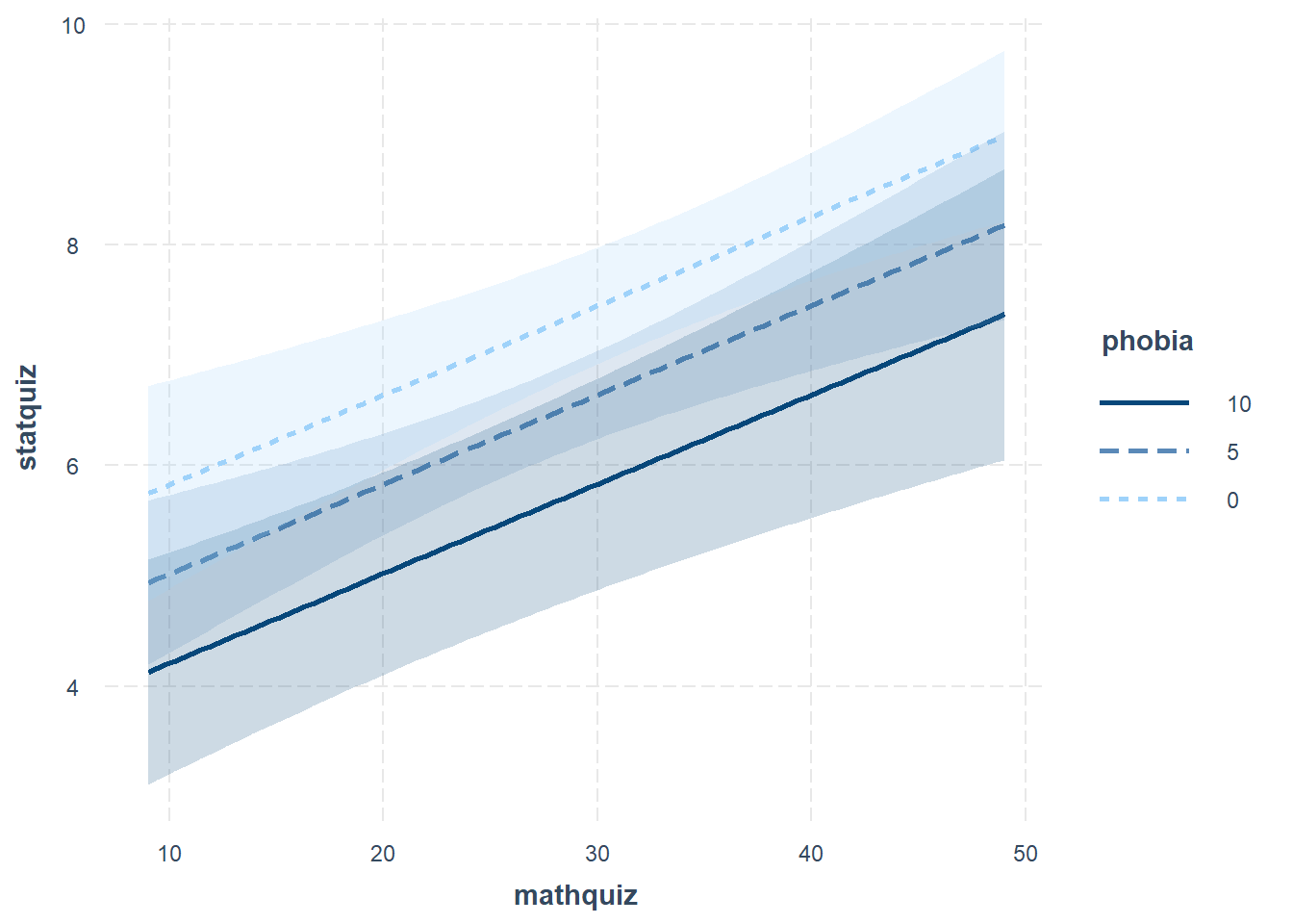
13.3.4 Visualize Relationships

When a model only contains main effects, a plot is not important for interpretation, but can help understand the relationship between multiple predictors.

interactions::interact_plot(model = fit_ihno_lm_3,
                            pred = mathquiz,
                            modx = phobia)

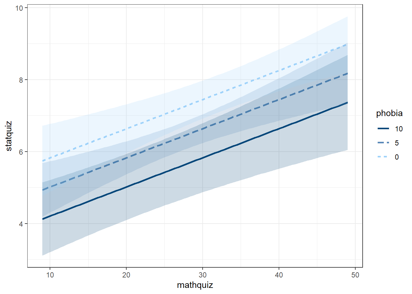
Interval = 95% Confidence Interval

interactions::interact_plot(model = fit_ihno_lm_3,
                            pred = mathquiz,
                            modx = phobia,
                            modx.values = c(0, 5, 10),
                            interval = TRUE)

Interval = plus-or-minus one standard error for the mean (SEM)

interactions::interact_plot(model = fit_ihno_lm_3,
                            pred = mathquiz,
                            modx = phobia,
                            modx.values = c(0, 5, 10),
                            interval = TRUE,
                            int.width = .68) +
  theme_bw()

interactions::interact_plot(model = fit_ihno_lm_3,
                            pred = phobia,
                            modx = mathquiz,
                            modx.values = c(15, 30, 45),
                            interval = TRUE,
                            int.width = .68) +
  theme_bw()

The Effect() function from the effects package chooses ‘5 or 6 nice values’ for each of your continuous independent variable (\(X's\)) based on the range of values found in the dataset on which the model and plugs all possible combinations of them into the regression equation \(Y = \beta_0 + \beta_1 X_1 + \beta_2 X_2 \dots \beta_k X_k\) to compute the predicted mean value of the outcome (\(Y\)) (Fox et al. 2022).

When plotting a regression model the outcome (dependent variable) is always on the y-axis (fit) and only one predictor (independent variable) may be used on the x-axis. You may incorporate additional predictor using colors, shapes, line types, or facets. For these predictors, you will want to specify only 2-4 values for illustration and then declare them as factors prior to plotting.

13.4 APA WRITE-UP

13.4.1 Methods

13.4.2 Results

There is evidence both mathquiz and phobia are associated with statquiz and that the relationship is addative (i.e. no interaction).

There is a strong association between math and stats quiz scores, r = .51. Math phobia is associated with lower math, r = -.28, and stats quiz scores, r = -.36. When considered together, the combined effects of math phobia and math score account for 31% of the variance in statistical achievement.

Not surprisingly, while higher self-reported math phobia was associated with lower statistics scores, b = -0.162, p = .018, 95% CI = [-0.29, -0.03], higher math quiz scores were associated with higher stats score, b = -0.081, p < .001, 95% CI = [0.05, 0.12].

There was no evidence that math phobia moderated the relationship between math and quiz performance, p = .377.

13.4.3 Table

Many journals prefer that regression tables include 95% confidence intervals, rater than standard errors for the beta estimates.

apaSupp::tab_lm(fit_ihno_lm_3,
                var_labels = c("mathquiz" = "Math Quiz",
                               "phobia" = "Math Phobia"),
                caption = "Multiple Linear Models for Statistics Quiz Performance Regressed on Math Phobia and Prior Math Performance",
                general_note = "Math Phobia was self-reported on a scale of 0 (none) to 10 (max) and the math quiz had a max of 50 points while the statistics quiz had a max of 10 points.",
                p_note = "* p < .05. *** p < .001.")

**Table 13.6**
Multiple Linear Models for Statistics Quiz Performance Regressed on Math Phobia and Prior Math Performance
Variable	b	(SE)	p	b*	𝜂²	𝜂ₚ²
(Intercept)	5.02	(0.63)	< .001 ***
Math Quiz	0.08	(0.02)	< .001 ***	0.44	.180	.206
Math Phobia	-0.16	(0.07)	.017 *	-0.23	.050	.067
R²	0.31
Adjusted R²	0.29
Note. Math Phobia was self-reported on a scale of 0 (none) to 10 (max) and the math quiz had a max of 50 points while the statistics quiz had a max of 10 points. b* = standardized estimate. 𝜂² = semi-partial correlation. 𝜂ₚ² = partial correlation.
* p < .05. *** p < .001.

13.4.4 Plot

effects::Effect(focal.predictors = c("mathquiz", "phobia"),
                mod = fit_ihno_lm_3,
                xlevels = list(phobia = c(0, 5, 10))) %>%   # values for illustration
  data.frame() %>% 
  dplyr::mutate(phobia = factor(phobia,
                                levels = c(0, 5, 10),
                                labels = c(" 0 = minimun",
                                           " 5 = middle",
                                           "10 = maximum"))) %>% # factor for illustration
  ggplot() +
  aes(x = mathquiz,
      y = fit,
      group = phobia) +
  geom_ribbon(aes(ymin = fit - se, 
                  ymax = fit + se),
              alpha = .15) +
  geom_line(aes(linetype = phobia),
            linewidth = 1) +
  theme_bw() +
  labs(x = "Score on Math Quiz",
       y = "Estimated Marginal Mean\nScore on Stat Quiz",
       linetype = "Self-Rated Math Phobia") +
  theme(legend.background = element_rect(color = "black"),
        legend.position = c(0, 1),
        legend.key.width = unit(2, "cm"),
        legend.justification = c(-0.1, 1.1)) +
  scale_linetype_manual(values = c("solid", "longdash", "dotted"))

Figure 13.10
Statistics Quiz Performance Regressed on Math Phobia and Prior Math Performance