Explaining Psychological Statistcs
A Compantion in R
Dr. Sarah Schwartz and Dr. Tyson Barrett
Updated Last: April 24 2018
USU: PSY 6600 -or- EDUC 6600
Utah State University Emma Eccles Jones College of Education and Human Services
This book is a compantion for the course text book:
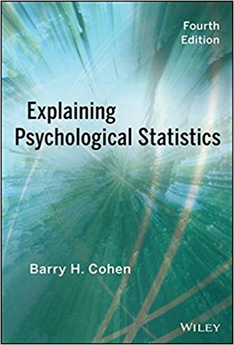
Cohen Textbook
The textbook is available through the USU library
- View and read it online for free
- You must be either on campus or on the VPN
- You will need to log-on with your A-number and password
- Download the entire book for free
- requires you to
- create an account with your A-number
- download/install some software
- only can be ‘checked out’ for 14 days
- requires you to
Course Files
All files may be downloaded from the BOX folder
Icons and image files (png or jpg)
Datasets (excel or SPSS format)
Assignments (pdf and Rmd)
Instructor Websites
Sarah’s website: www.sarahschwartzstats.com
Tyson’s website: www.tysonbarrett.com/teaching/
Other Websites
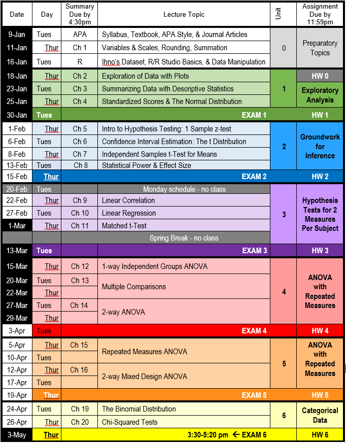
| Course Schedule |
| For Spring Semester 2018 |
 |
| # COMPUTER PREPARATION {-} |
 |
| What is R? |
| R is a language and environment for statistical computing and graphics. (R Core Team 2017) |
| R provides a wide variety of statistical (linear and nonlinear modelling, classical statistical tests, time-series analysis, classification, clustering, …) and graphical techniques, and is highly extensible. The S language is often the vehicle of choice for research in statistical methodology, and R provides an Open Source route to participation in that activity. |
| One of R’s strengths is the ease with which well-designed publication-quality plots can be produced, including mathematical symbols and formulae where needed. Great care has been taken over the defaults for the minor design choices in graphics, but the user retains full control. |
| What is R Markdown? |
| According to R Studio: |
| > “R Markdown is a format that enables easy authoring of reproducible web reports from R. It combines the core syntax of Markdown (an easy-to-write plain text format for web content) with embedded R code chunks that are run so their output can be included in the final document”. |
Dynamic Reporting
From Penn State Statistics:
The traditional way** to write a report**
- Run your analysis in software, like SPSS or R and manually save our output
- i.e. saving the ANOVA table or using pdf() to save the graphs
- Type your your description and interpretation in a text editor like Word
- either drag/drop tables and figures, or worse copy-paste and retype all the numbers
A report written in this way can be problematic. For instance, imagine your Mentor/collaborator/journal reviewer telling you that they want to use a sub-sample instead of the entire sample. Or to include a nother variable. You would have to redo all of your work!!
Therefore, in this way dynamic also means reproducible, in the sense that people who get the file from you can reproduce the entire work in the report.
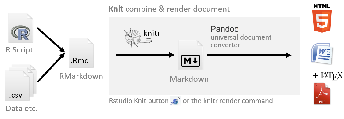
How does R Markdown work out to be a .pdf or .html file?
R Markdown is a file with the file extension .Rmd, the knitr package will then transform the file into a Markdown file with the extension .md. Then Rstudio can (Xie 2015):
Use
LaTeXto transform the file into a .pdfLoad another package called
markdownto transform the file into .htmlUse Pandoc to even convert to file to a Word document (ugly)
Is this a popular** method for creating reports?**
Check out Rpubs. This website shares lots of documents written in the way we will introduce below.
R Markdowndocuments are fully reproducible. Use a productive notebook interface to weave together narrative text and code to produce elegantly formatted output. Use multiple languages including R, Python, and SQL (Allaire et al. 2017).

knitris an engine for dynamic report generation with R. It is a package in the statistical programming language R that enables integration of R code into LaTeX, LyX, HTML, Markdown, AsciiDoc, and text documents (Xie 2017b).
Software Programs
You will need to download and install THREE programs to create dynamic reports in.

1. R from www.r-project.org
Get the latest released version of FREE Base R from CRAN
- Choose a mirror close to your location
- Select base R for your computer (Windows, Mac, ect.)
- The defaults are good…don’t change them…just keep clicking ‘Next’

2 R Studio from www.rstudio.com
Get the latest version of the FREE Open Source Desktop Edition of R Studio
- The defaults are good…don’t change them…just keep clicking ‘Next’

3. LaTeX depends on your operating system
Mac:
MacTeXfrom http://tug.org/mactex/
- Download (5+ min) to a folder and them double click on the PKG file
- Follow the installation instructions.
- You don’t need to open anything after MacTeX is finished installing.
Windows:
MikTeXhttp://miktex.org/download
- Pick the latest version of the Net Installer, not the Basic!
- You need the full version 64-bit is better, if you have a 64-bit machine
- When your download is complete, run the downloaded installer.
- Windows may ask you if you want to “allow this app from an unknown publisher to make changes to your PC”. If it does, make sure to click Yes!
- This is the slowest part…
R Packages
R packages are collections of functions and data sets developed by the community. They increase the power of R by improving existing base R functionalities, or by adding new ones.
More information may be found here: https://www.datacamp.com/community/tutorials/r-packages-guide
0.0.1 Packages You Need!
The followin packages are used in this course and throught this document:
Installing Packages (via the user interface)
You only need to install packages ONCE per computer.
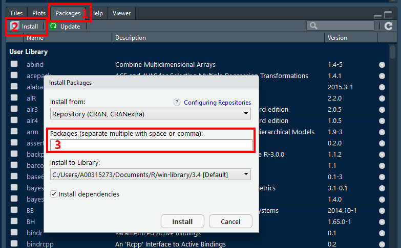
In R Stuido:
- Click on the Packages tab the panel with the most tabs
- Click on the word Instsall just under and to the left of the tab
- In the Packages box, type in the name of the packages you would like to download. You can do several at once, just seperate them with multiple spaces or a comma.
Note: Leave the installation library path as the default. Also, make sure the box for ‘Installing dependencies’ is checked.
Load Packages (via code)
You will need to load packages in EVERY SESSION you want to use them in.
library(tidyverse)Please don’t get confused: library() is the command used to load a package, and it refers to the place where the package is contained, usually a folder on your computer, while a package is the collection of functions bundled conveniently.
Maybe it can help a quote from Hadley Wickham, Chief data scientist at RStudio, and instructor of the “Writing functions in R” DataCamp course (December 8, 2014):
“a package is a like a book, a library is like a library; you use
library()to check a package out of the library”
Here is link to an AWSOME ‘cheat sheet’ for begginers working with the tidyverse package. I highly suggest checking it out.
More ‘cheat sheets’ are available under the “Help” menu option in R Studio
Kniting Notebooks
Storing all associated files
If you are using any files, such as datasets or images, they need to be stored in the same folder location as the R Notebook (.Rmd file).
This folder location must be the Working Directory for the R Studio session. If you opened your .Rmd notebook file by double-clicking on its name, then this should be the case.
Setting the working directory
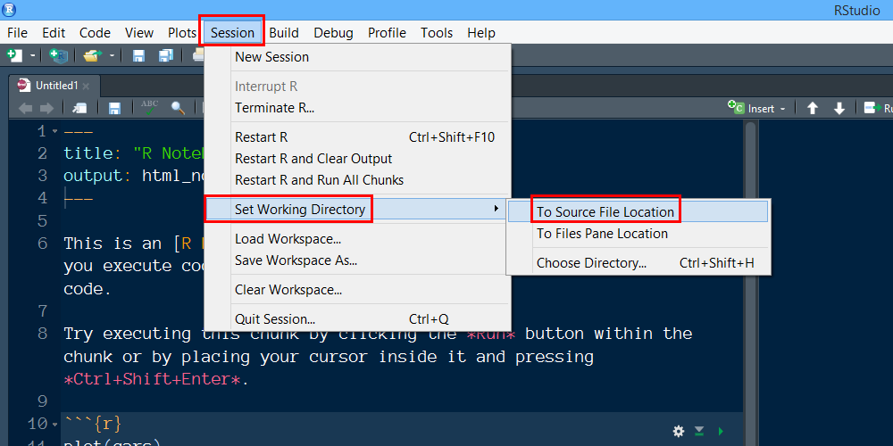
To ensure that R Studio knows where to find the files, you can manually set the Working Directory through the menu:
- Click
Session - Select
Set Working Directoryby hovering your mouse over it - Click on
To Source File Location
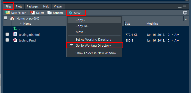
You can double check that you were successful by
- Click on the
Filestab in the many-tab panel - Click on the button with the gear that says
More - Click
Go To Working Directory
At this point you should see all the files that reside in the folder location where the open .Rmd files is also saved.