Chapter 7 t TEST FOR THE DIFFERENCE IN 2 MEANS, INDEPENDENT SAMPLES
Chapter Links
Assignment Links
Required Packages
library(tidyverse)    # Loads several very helpful 'tidy' packages
library(haven)        # Read in SPSS datasets
library(car)          # Companion for Applied Regression (and ANOVA)
Example: Cancer Experiment
The Cancer dataset was introduced in chapter 3.
Check Means and SD’s
cancer_clean %>%
  dplyr::group_by(trt) %>%
  furniture::table1(totalcin, totalcw4)
--------------------------------
                 trt
          Placebo    Aloe Juice
          n = 14     n = 11
 totalcin
          6.6 (0.9)  6.5 (2.1)
 totalcw4
          10.1 (3.6) 10.6 (3.5)
--------------------------------
7.1 Assumtion Check: Eyeball method
Do the two groups, treatment and control, have the same amount of spread (standard deviations) BUT different centers (means)?
cancer_clean %>%
  ggplot(aes(x = trt,
             y = totalcin)) +
  geom_boxplot()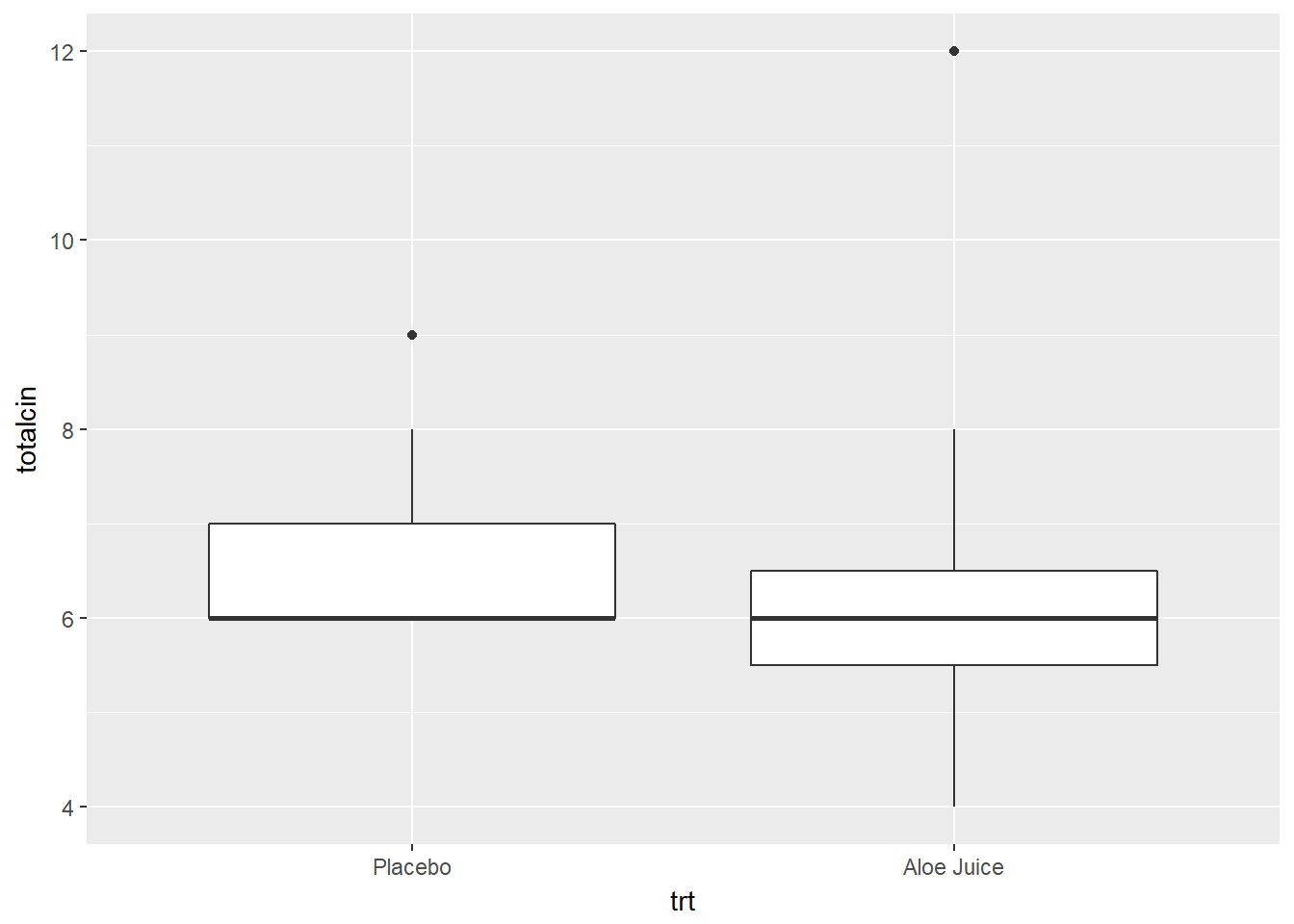
cancer_clean %>%
  ggplot(aes(x = trt,
             y = totalcw4)) +
  geom_boxplot()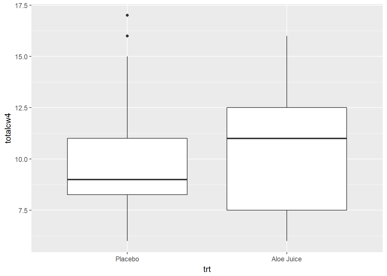
7.2 Assumtion Check: Homogeneity of Variance
Before performing the \(t\) test, check to see if the assumption of homogeneity of variance is met using Levene’s Test. For a independent samples t-test for means, the groups need to have the same amount of spread (SD) in the measure of interest.
Use the car:leveneTest() function to do this. Inside the funtion you need to specify at least three things (sepearated by commas):
- the formula:
continuous_var ~ grouping_var(replace with your variable names) - the dataset:
data = .to pipe it from above - the center:
center = "mean"since we are comparing means
Do the participants in the treatment and control groups have the same spread in oral condition at BASELINE?
cancer_clean %>%
  car::leveneTest(totalcin ~ trt,    # formula: continuous_var ~ grouping_var
                  data = .,          # pipe in the dataset
                  center = "mean")   # The default is "median"
Levene's Test for Homogeneity of Variance (center = "mean")
Df F value Pr(>F)
group 1 2.2103 0.1507
23 No violations of homogeneity were detected, \(F(1, 23) = 2.210, p = .151\).
Do the participants in the treatment and control groups have the same spread in oral condition at the FOURTH WEEK?
cancer_clean %>%
  car::leveneTest(totalcw4 ~ trt,    # formula: continuous_var ~ grouping_var
                  data = .,          # pipe in the dataset
                  center = "mean")   # The default is "median"
Levene's Test for Homogeneity of Variance (center = "mean")
Df F value Pr(>F)
group 1 0 0.995
23 No violations of homogeneity were detected, \(F(1, 23) = 0, p = .995\).
7.3 2 independent Sample Means
Use the same t.test() funtion we have used in the prior chapters. This time you need to speficy a few more options.
the formula:
continuous_var ~ grouping_var(replace with your variable names)the dataset:
data = .to pipe it from aboveis homogeneity satified?:
var.equal = TRUE(NOT the default)number of tails:
alternative = "two.sided"independent vs. paired:
paired = FALSEconfidence level:
conf.level = #
Do the participants in the treatment group have a different average oral condition at BASELINE, compared to the control group?
# Minimal syntax
cancer_clean %>%
  t.test(totalcin ~ trt,   # formula: continuous_var ~ grouping_var
         data = .,         # pipe in the dataset
         var.equal = TRUE) # HOV was violated (option = TRUE)
    Two Sample t-test

data:  totalcin by trt
t = 0.18566, df = 23, p-value = 0.8543
alternative hypothesis: true difference in means is not equal to 0
95 percent confidence interval:
 -1.185479  1.419245
sample estimates:
   mean in group Placebo mean in group Aloe Juice
                6.571429                 6.454545
No evidence of a differnece in mean oral condition at baseline, \(t(23) = 0.186, p = .854\).
Do the participants in the treatment group have a different average oral condition at the FOURTH WEEK, compared to the control group?
# Fully specified function
cancer_clean %>%
  t.test(totalcw4 ~ trt,             # formula: continuous_var ~ grouping_var
         data = .,                   # pipe in the dataset
         var.equal = TRUE,           # default: HOV was violated (option = TRUE)
         alternative = "two.sided",  # default: 2 sided (options = "less", "greater")
         paired = FALSE,             # default: independent (option = TRUE)
         conf.level = .95)           # default: 95% (option = .9, .90, ect.)
    Two Sample t-test

data:  totalcw4 by trt
t = -0.34598, df = 23, p-value = 0.7325
alternative hypothesis: true difference in means is not equal to 0
95 percent confidence interval:
 -3.444215  2.457202
sample estimates:
   mean in group Placebo mean in group Aloe Juice
                10.14286                 10.63636
No evidence of a differnece in mean oral condition at the fourth week, \(t(23) = -0.350, p = .733\).