Chapter 9 Linear Correlation

Chapter Links

Unit Assignment Links

Unit 3 Writen Part: Skeleton - pdf
Unit 3 R Part: Directions - pdf and Skeleton - Rmd
Unit 3 Reading to Summarize: Article - pdf
Inho’s Dataset: Excel

Required Packages

library(tidyverse)    # Loads several very helpful 'tidy' packages
library(haven)        # Read in SPSS datasets
library(psych)        # Lots of nice tid-bits
library(GGally)       # Extension to 'ggplot2' (ggpairs)

Example: Cancer Experiment

The Cancer dataset was introduced in chapter 3.

9.1 Visualize the Raw Data

Always plot your data first!

cancer_clean %>% 
  ggplot(aes(x = age,
             y = weighin)) +
  geom_point() +
  geom_smooth(method = "lm")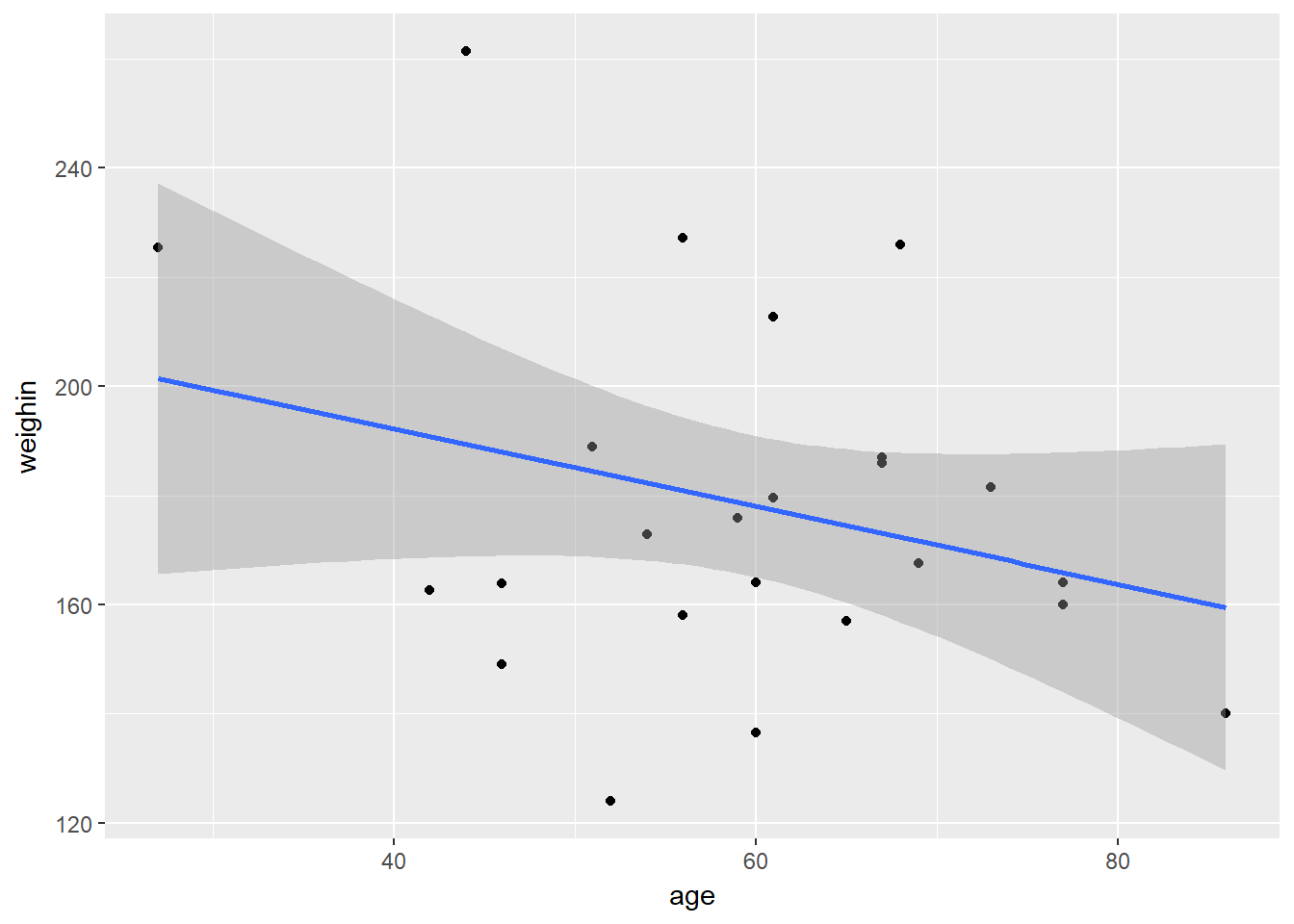

9.2 Pearson’s Correlation Coefficient

The cor.test() function needs at least TWO arguments:

formula - The formula specifies the two variabels between which you would like to calcuate the correlation. Note at the two variable names come AFTER the tilda symbol and are separated with a plus sign: ~ continuous_var1 + continuous_var2
data - Since the datset is not the first argument in the function, you must use the period to signify that the datset is being piped from above data = .

cancer_clean %>% 
  cor.test(~ age + weighin,  # formula: order doesn't matter
           data = .)         # data piped from above


    Pearson's product-moment correlation

data:  age and weighin
t = -1.4401, df = 23, p-value = 0.1633
alternative hypothesis: true correlation is not equal to 0
95 percent confidence interval:
 -0.6130537  0.1213316
sample estimates:
       cor 
-0.2875868

9.2.1 Additional Arguments

alternative - The cor.test() function defaults to the alternative = "two.sided". If you would like a one-sided alternative, you must choose which side you would like to test: alternative = "greater" to test for POSITIVE correlation or alternative = "less" to test for NEGATIVE correlation.
method - The default is to calculate the Pearson correlation coefficient (method = "pearson"), but you may also specify the Kendall’s tau (method = "kendall")or Spearman’s rho (method = "spearman"), which are both non-parametric methods.
conf.int - It also defaults to testing for the two-sided alternative and computing a 95% confidence interval (conf.level = 0.95), but this may be changed.

Since the following code only specifies thedefaults, it Will give the same results as if you did not type out the last three lines (see above).

cancer_clean %>% 
  cor.test(~ age + weighin,
           data = .,
           alternative = "two.sided",  # or "greater" (positive r) or "less" (negative r)
           method = "pearson",          # or "kendall" (tau) or "spearman" (rho)
           conf.level = .95)            # or .90 or .99 (ect)


    Pearson's product-moment correlation

data:  age and weighin
t = -1.4401, df = 23, p-value = 0.1633
alternative hypothesis: true correlation is not equal to 0
95 percent confidence interval:
 -0.6130537  0.1213316
sample estimates:
       cor 
-0.2875868

9.2.2 Statistical Significance

Non-Significant Correlation

APA Results: There was no evidence of an association in overall oral condition from baseline to two week follow-up, $r(25) = -0.288 $p < .163$.

cancer_clean %>% 
  ggplot(aes(x = totalcin,
             y = totalcw4)) +
  geom_point() +
  geom_smooth(method = "lm")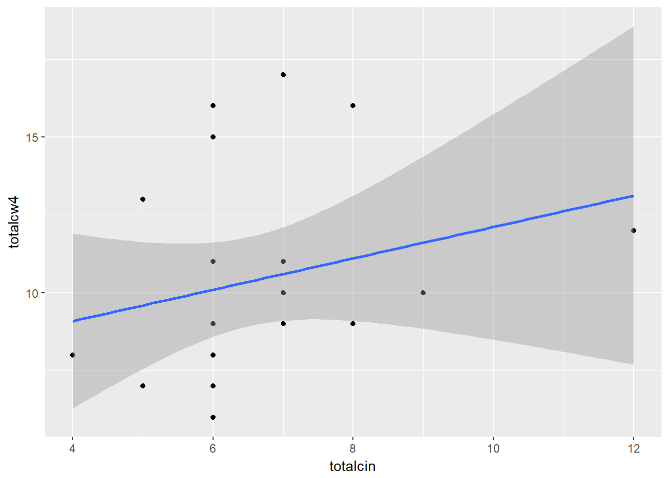

cancer_clean %>% 
  cor.test(~ totalcin + totalcw4,
           data = .)


    Pearson's product-moment correlation

data:  totalcin and totalcw4
t = 1.0911, df = 23, p-value = 0.2865
alternative hypothesis: true correlation is not equal to 0
95 percent confidence interval:
 -0.1899343  0.5672525
sample estimates:
      cor 
0.2218459

Statistically Significant Correlation

APA Results: Overall oral condition was positively correlated ($r = .763$) between weeks two and four, $t(21) = 5.409$, $p < .001$.

cancer_clean %>% 
  ggplot(aes(x = totalcw4,
             y = totalcw6)) +
  geom_point() +
  geom_smooth(method = "lm")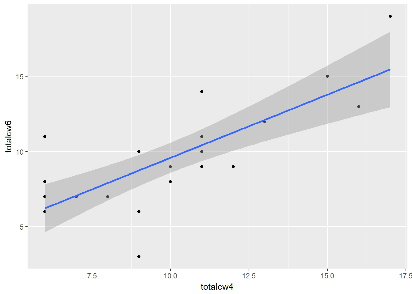

cancer_clean %>% 
  cor.test(~ totalcw4 + totalcw6,
           data = .)


    Pearson's product-moment correlation

data:  totalcw4 and totalcw6
t = 5.4092, df = 21, p-value = 2.296e-05
alternative hypothesis: true correlation is not equal to 0
95 percent confidence interval:
 0.5117459 0.8940223
sample estimates:
     cor 
0.762999

9.3 Correlation Tables

The may use the tableC() function from the furniture package to calculate all pair-wise correlations between more than two variables and arrange them all in a table. The table is formatted with the variabels listed on the rows and numbered to show the same variabels across the columns.

The cells ON the diagonal are all equal to exactly one, since each variable is perfectly correlated with itself.
The cells ABOVE the diagonal are blank as them would just be a mirror image of the values below the diagonal.
The cells BELOW the diagonal each contain the Pearson’s correlation coefficients for each pair of variables, $r$, with the $p-value$ showing the significance vs. the null hypothesis for no association ($r = 0$) to the right.

cancer_clean %>% 
  furniture::tableC(age, weighin, totalcin)


-----------------------------------------------
             [1]            [2]          [3]  
 [1]age      1.00                             
 [2]weighin  -0.288 (0.163) 1.00              
 [3]totalcin 0.256 (0.217)  0.17 (0.418) 1.00 
-----------------------------------------------

9.3.1 Missing Values - Default

Default Behavior na.rm = FALSE (default)

If you don’t say otherwise, the correlation $r$ with not be calculated (NA) between any pair of variables for which there is at least one subject with a missing value on at least one of the vairables. This is a nice alert to make you aware of missing values.

cancer_clean %>% 
  furniture::tableC(totalcin, totalcw2, totalcw4, totalcw6)


-----------------------------------------------------
             [1]           [2]           [3]   [4]  
 [1]totalcin 1.00                                   
 [2]totalcw2 0.314 (0.126) 1.00                     
 [3]totalcw4 0.222 (0.287) 0.337 (0.099) 1.00       
 [4]totalcw6 NA NA         NA NA         NA NA 1.00 
-----------------------------------------------------

9.3.2 Missing Values - Listwise Deletion

Listwise Deletion na.rm = TRUE

Most of the time you will want to compute the correlation $r$ is the precense of missing values. To do so, you want to remove or exclude subjects with missing data from ALL correlation computation in the table. This is called ‘list-wise deletion’. It ensures that all cells in the table refer to the exact same sub-sample (n = subjects with complete data for all variables in the table), and thus the same degrees of freedom (since $df = n - 2$). This is done be changing the default to na.rm = TRUE.

cancer_clean %>% 
  furniture::tableC(totalcin, totalcw2, totalcw4, totalcw6,
                    na.rm = TRUE)


-------------------------------------------------------------
             [1]           [2]           [3]           [4]  
 [1]totalcin 1.00                                           
 [2]totalcw2 0.282 (0.192) 1.00                             
 [3]totalcw4 0.206 (0.346) 0.314 (0.145) 1.00               
 [4]totalcw6 0.098 (0.657) 0.378 (0.075) 0.763 (<.001) 1.00 
-------------------------------------------------------------

9.4 Pairs Plots

Helpful Website

9.4.1 Base R

cancer_clean %>% 
  dplyr::select(age, weighin, 
                totalcin, totalcw2, totalcw4, totalcw6) %>% 
  pairs()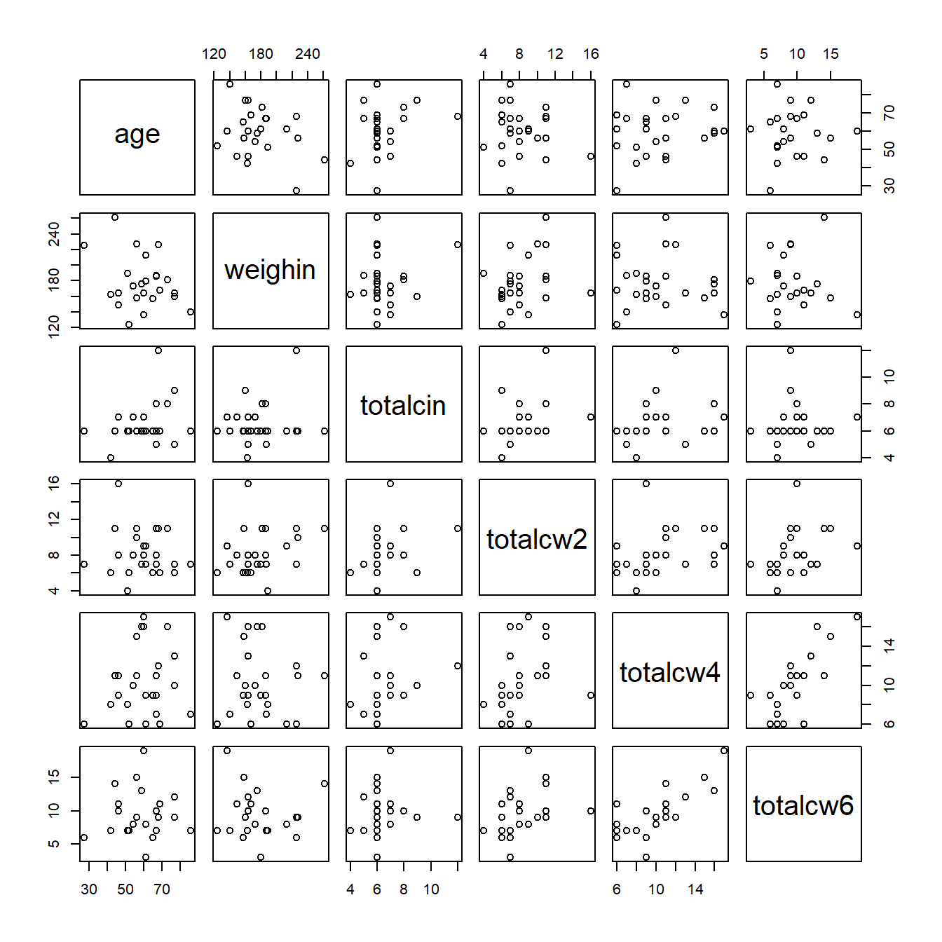

9.4.2 `psych` package

cancer_clean %>% 
  dplyr::select(age, weighin,
                totalcin, totalcw2, totalcw4, totalcw6) %>% 
  psych::pairs.panels()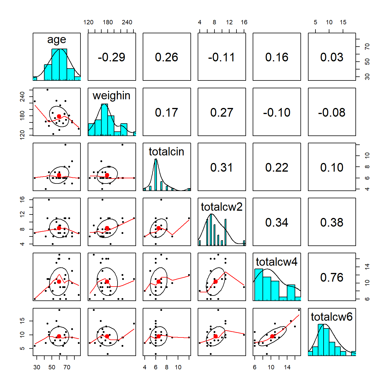

9.4.3 `ggplot2` and `GGally` packages

cancer_clean %>% 
  dplyr::select(age, weighin,
                totalcin, totalcw2, totalcw4, totalcw6) %>% 
  data.frame %>% 
  ggscatmat()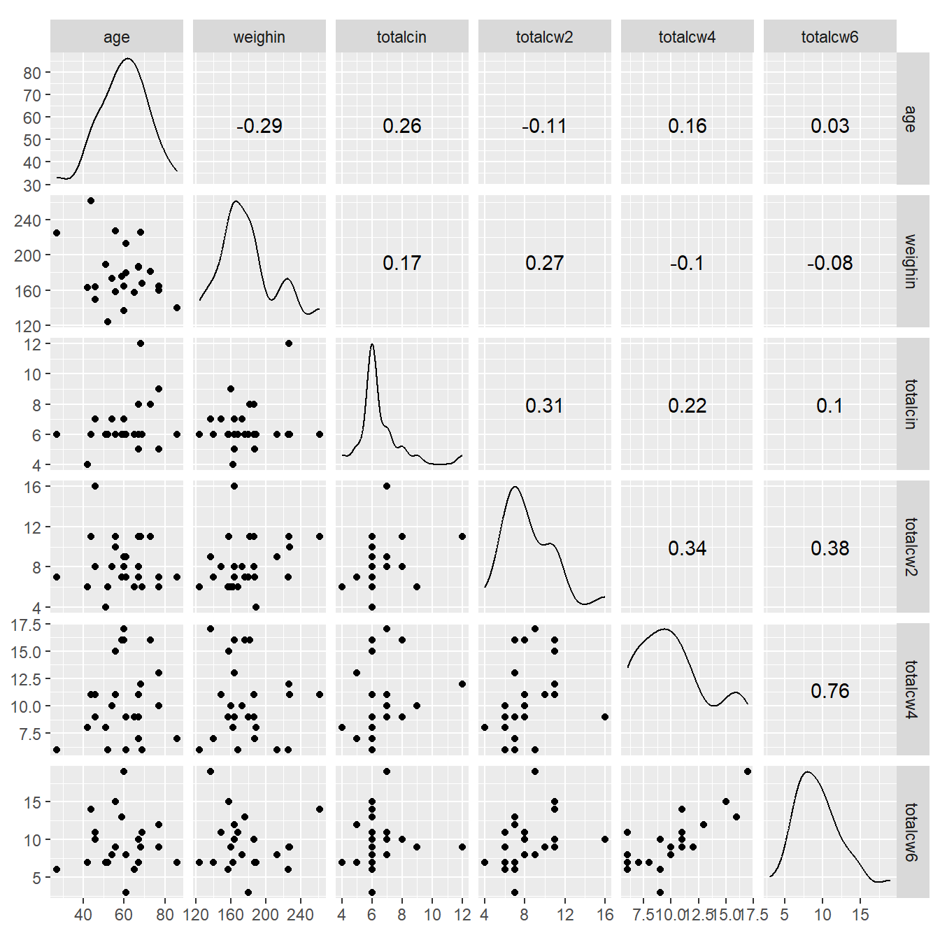

cancer_clean %>% 
  data.frame %>% 
  ggscatmat(columns = c("age", "weighin",
                        "totalcin", "totalcw2", "totalcw4", "totalcw6"),
            color = "trt")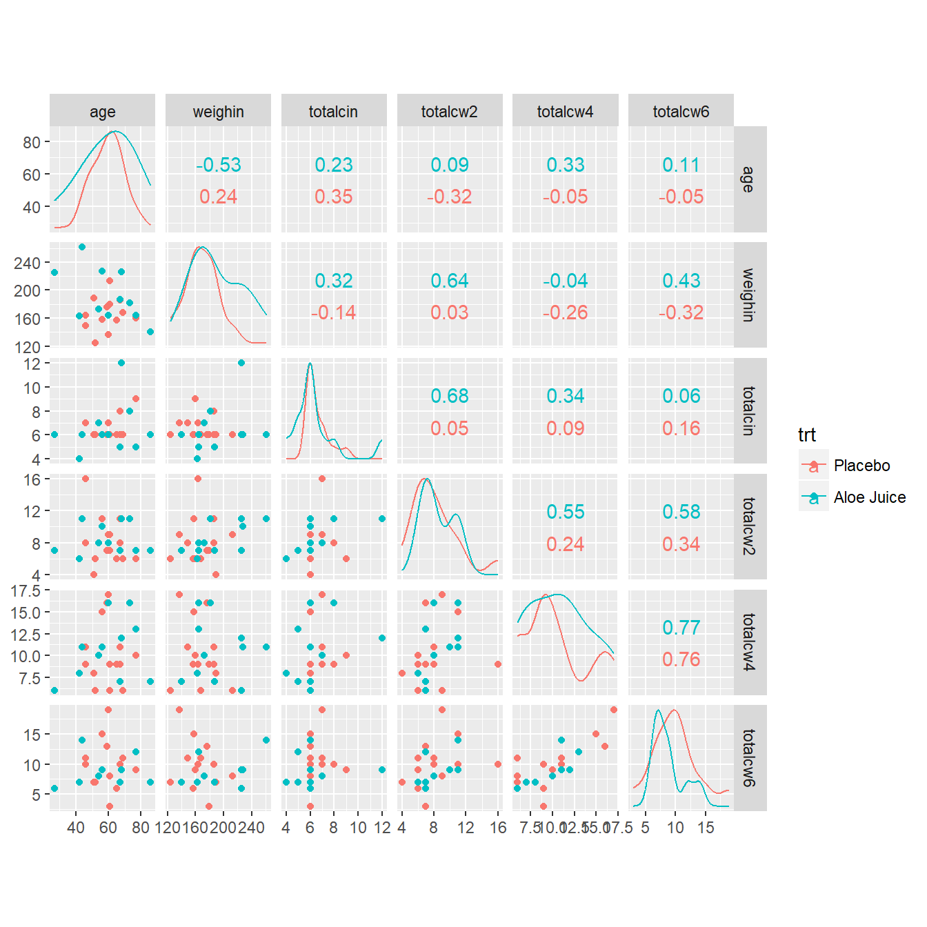

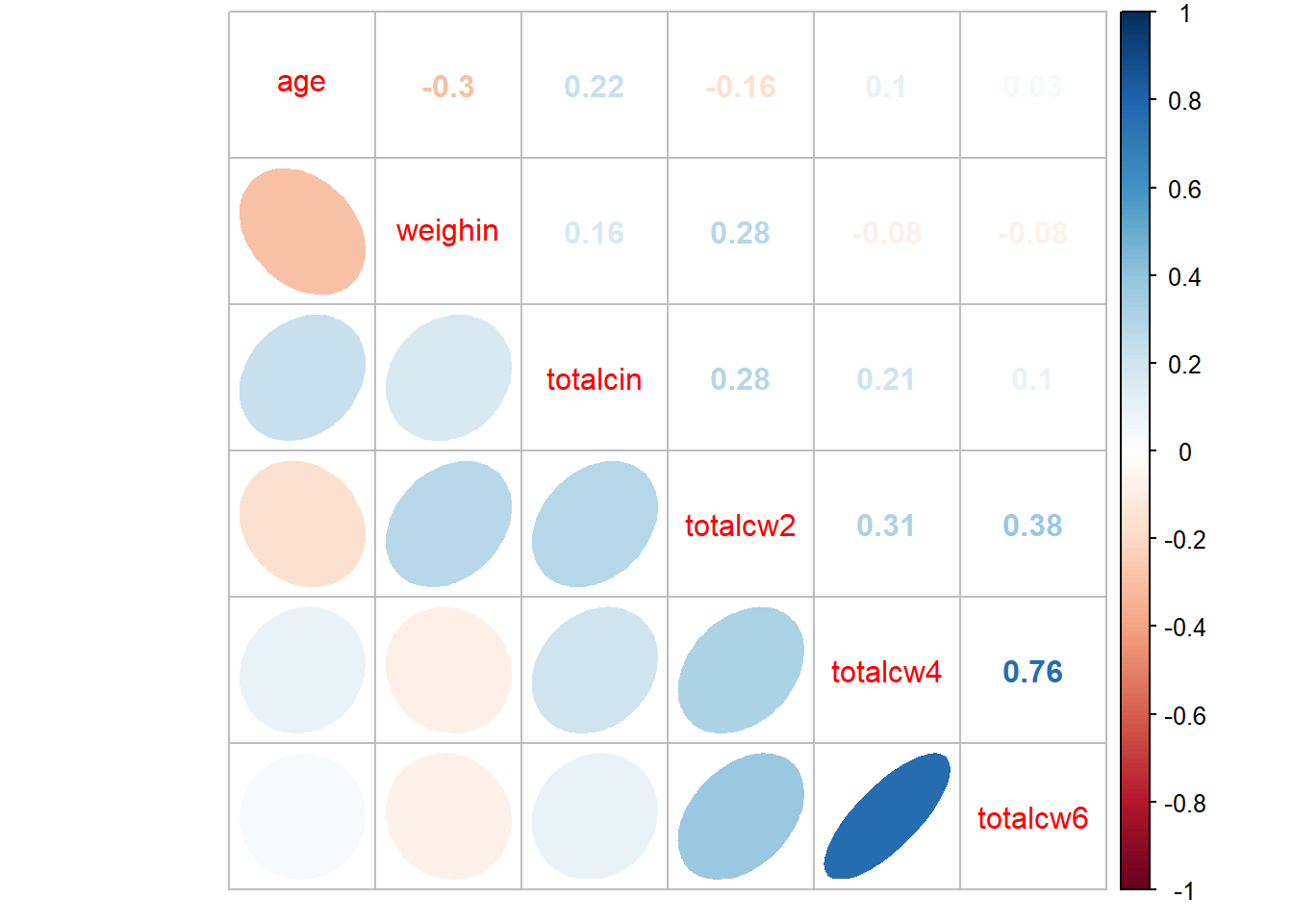
9.5 Correlation Plots: Corrolagrams

cancer_clean %>% 
  dplyr::select(age, weighin, 
                totalcin, totalcw2, totalcw4, totalcw6) %>% 
  cor(method = "pearson",
      use = "complete.obs")

                 age     weighin   totalcin   totalcw2    totalcw4
age       1.00000000 -0.29909121 0.22386540 -0.1613892  0.09918029
weighin  -0.29909121  1.00000000 0.16403694  0.2763478 -0.08013506
totalcin  0.22386540  0.16403694 1.00000000  0.2819648  0.20604650
totalcw2 -0.16138924  0.27634783 0.28196479  1.0000000  0.31354250
totalcw4  0.09918029 -0.08013506 0.20604650  0.3135425  1.00000000
totalcw6  0.03015273 -0.07750304 0.09786664  0.3780949  0.76299899
            totalcw6
age       0.03015273
weighin  -0.07750304
totalcin  0.09786664
totalcw2  0.37809488
totalcw4  0.76299899
totalcw6  1.00000000

cancer_clean %>% 
  dplyr::select(age, weighin, 
                totalcin, totalcw2, totalcw4, totalcw6) %>% 
  cor(method = "pearson",
      use = "complete.obs") %>% 
  corrplot::corrplot()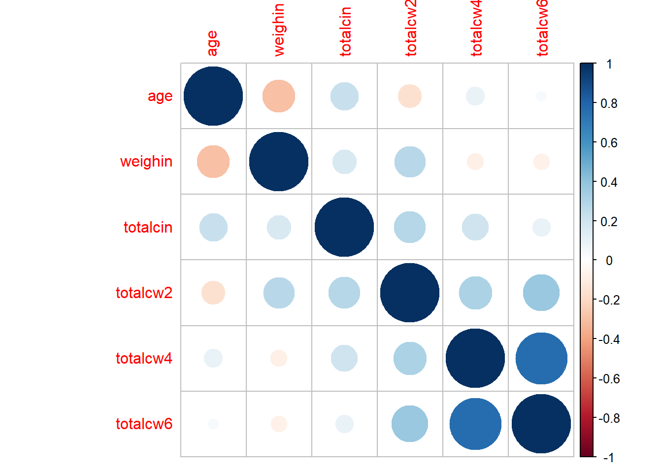

cancer_clean %>% 
  dplyr::select(age, weighin, 
                totalcin, totalcw2, totalcw4, totalcw6) %>% 
  cor(method = "pearson",
      use = "complete.obs") %>% 
  corrplot::corrplot(method = "square")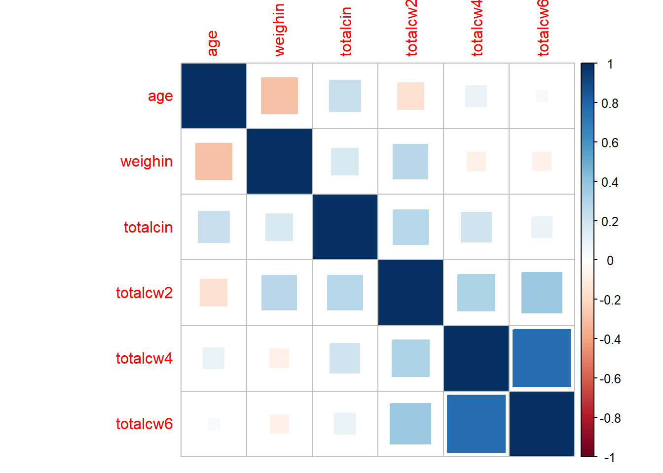

cancer_clean %>% 
  dplyr::select(age, weighin, 
                totalcin, totalcw2, totalcw4, totalcw6) %>% 
  cor(method = "pearson",
      use = "complete.obs") %>% 
  corrplot::corrplot(method = "ellipse",
                     type = "lower")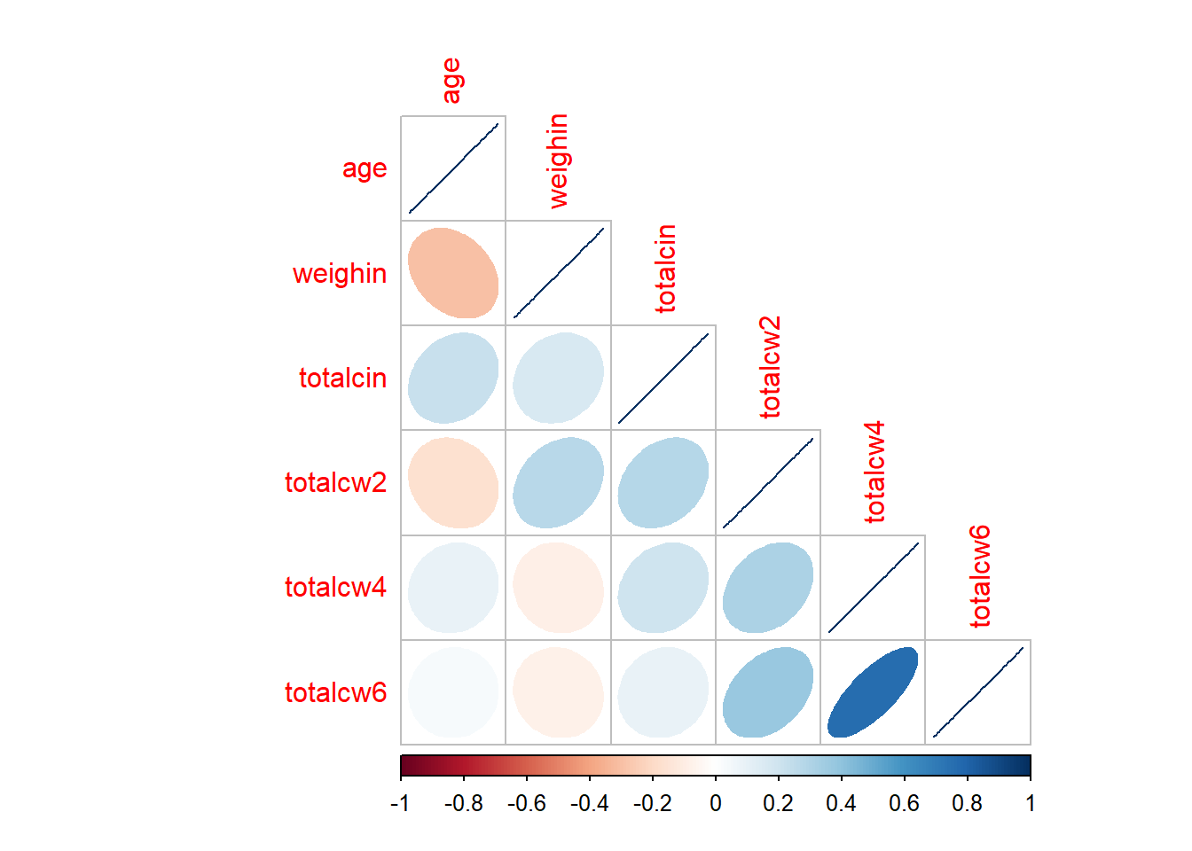

cancer_clean %>% 
  dplyr::select(age, weighin, 
                totalcin, totalcw2, totalcw4, totalcw6) %>% 
  cor(method = "pearson",
      use = "complete.obs") %>% 
  corrplot::corrplot.mixed()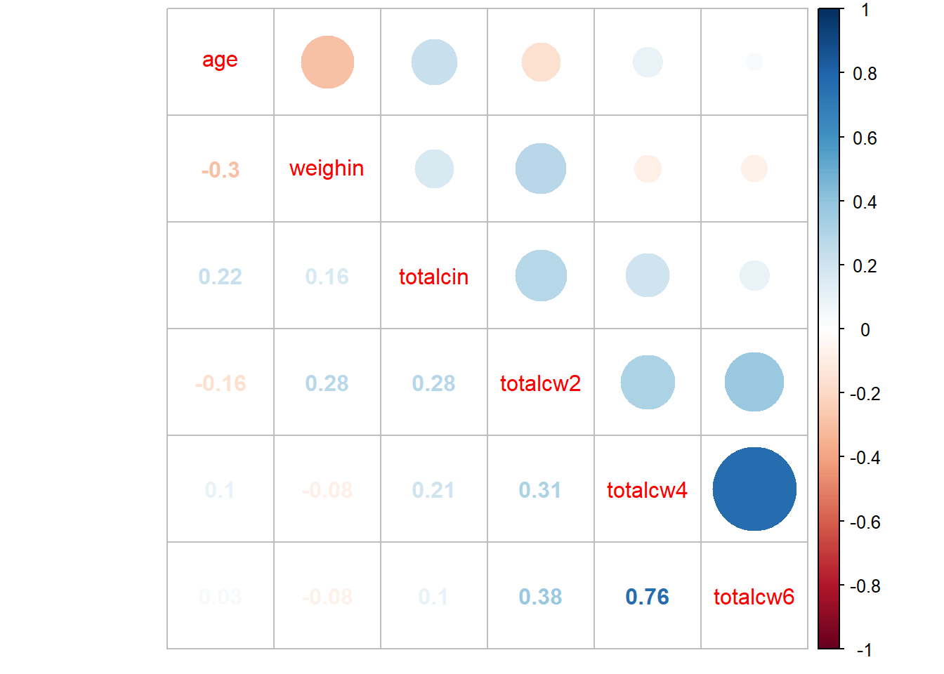

cancer_clean %>% 
  dplyr::select(age, weighin, 
                totalcin, totalcw2, totalcw4, totalcw6) %>% 
  cor(method = "pearson",
      use = "complete.obs") %>% 
  corrplot::corrplot.mixed(upper = "number",
                           lower = "ellipse")