Chapter 10 Linear Regression

Chapter Links

Unit Assignment Links

Unit 3 Writen Part: Skeleton - pdf
Unit 3 R Part: Directions - pdf and Skeleton - Rmd
Unit 3 Reading to Summarize: Article - pdf
Inho’s Dataset: Excel

Related Readings

Required Packages

library(tidyverse)    # Loads several very helpful 'tidy' packages
library(haven)        # Read in SPSS datasets
library(car)          # Companion for Applied Regression (and ANOVA)
library(broom)        # Convert STatistical Analysis Objects into Tidy Dataframes
library(magrittr)     # A Forward-Pipe Operator for R

Example: Cancer Experiment

The Cancer dataset was introduced in chapter 3.

10.1 Visualize the Raw Data

Always plot your data first!

cancer_clean %>% 
  ggplot(aes(x = age,
             y = weighin)) +
  geom_point() +
  geom_smooth(method = "lm",    se = TRUE, color = "blue") +  # straight line (linear model)
  geom_smooth(method = "loess", se = FALSE, color = "red")   # loess line (moving window)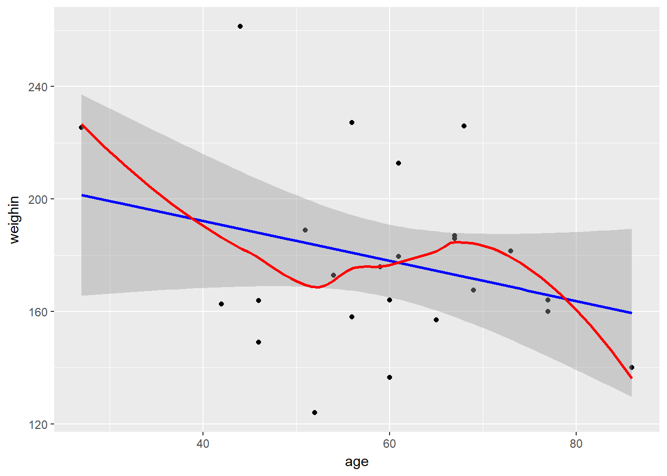

10.2 Fitting a Simple Regression Model

The lm() function needs at least TWO arguments:

formula - The name of the outcome or dependent variable (DV) goes on the left of the tilda symbol and the name of the predictor or independent variable (IV) comes after: continuous_y ~ continuous_x
data - Since the datset is not the first argument in the function, you must use the period to signify that the datset is being piped from above data = .

cancer_clean %>% 
  lm(weighin ~ age,    # formula: order DOES matter
     data = .)         # data piped from above


Call:
lm(formula = weighin ~ age, data = .)

Coefficients:
(Intercept)          age  
   220.6899      -0.7111

10.3 Extracting Information From the Model

10.3.1 Model Overview

To view more complete information, add a summary() step using a pipe AFTER the lm() step

cancer_clean %>% 
  lm(weighin ~ age,    # formula: order DOES matter
     data = .) %>%     # data piped from above
  summary()


Call:
lm(formula = weighin ~ age, data = .)

Residuals:
    Min      1Q  Median      3Q     Max 
-59.713 -19.535  -2.935  12.954  71.998 

Coefficients:
            Estimate Std. Error t value Pr(>|t|)    
(Intercept) 220.6899    30.1076    7.33 1.86e-07 ***
age          -0.7111     0.4938   -1.44    0.163    
---
Signif. codes:  0 '***' 0.001 '**' 0.01 '*' 0.05 '.' 0.1 ' ' 1

Residual standard error: 31.28 on 23 degrees of freedom
Multiple R-squared:  0.08271,   Adjusted R-squared:  0.04282 
F-statistic: 2.074 on 1 and 23 DF,  p-value: 0.1633

NOTE - Variable Designation Matters!

In simple linear regression (with only one predictor DV), the slope estimate (\(\hat{\beta_1}\)) is different depending on the designation of \(x\) and \(y\) (two ordering), but the \(p-values\) are the same.

cancer_clean %>% 
  lm(age ~ weighin,    # formula: order DOES matter
     data = .) %>%     # data piped from above
  summary()


Call:
lm(formula = age ~ weighin, data = .)

Residuals:
    Min      1Q  Median      3Q     Max 
-27.160  -6.277   1.514   8.258  21.908 

Coefficients:
            Estimate Std. Error t value Pr(>|t|)    
(Intercept) 80.37531   14.61964   5.498 1.37e-05 ***
weighin     -0.11631    0.08077  -1.440    0.163    
---
Signif. codes:  0 '***' 0.001 '**' 0.01 '*' 0.05 '.' 0.1 ' ' 1

Residual standard error: 12.65 on 23 degrees of freedom
Multiple R-squared:  0.08271,   Adjusted R-squared:  0.04282 
F-statistic: 2.074 on 1 and 23 DF,  p-value: 0.1633

10.3.2 Model Fit or Accuracy

One line for the entire model

cancer_clean %>% 
  lm(weighin ~ age,    
     data = .) %>%     
  broom::glance()

   r.squared adj.r.squared    sigma statistic   p.value df    logLik
1 0.08270615    0.04282381 31.28435  2.073754 0.1633263  2 -120.5091
       AIC      BIC deviance df.residual
1 247.0183 250.6749 22510.34          23

10.3.3 Beta Estimates

One line for each parameter, intercept and a slope for each predictor

cancer_clean %>% 
  lm(weighin ~ age,    
     data = .) %>%     
  broom::tidy()

         term    estimate  std.error statistic      p.value
1 (Intercept) 220.6899336 30.1075690  7.330048 1.859355e-07
2         age  -0.7110988  0.4938003 -1.440053 1.633263e-01

10.3.4 Confidence Intervals

cancer_clean %>% 
  lm(weighin ~ age,    
     data = .) %>%     
  confint()

                 2.5 %     97.5 %
(Intercept) 158.407682 282.972185
age          -1.732603   0.310405

10.3.5 Predictions, Residuals, ect.

One line for each subject in the original dataset

cancer_clean %>% 
  lm(weighin ~ age,    
     data = .) %>%     
  broom::augment()

   weighin age  .fitted   .se.fit     .resid       .hat   .sigma
1    124.0  52 183.7128  7.306243 -59.712795 0.05454237 29.18516
2    160.0  77 165.9353 10.612917  -5.935324 0.11508411 31.95915
3    136.5  60 178.0240  6.259394 -41.524004 0.04003229 30.68475
4    179.6  61 177.3129  6.292807   2.287094 0.04046081 31.98358
5    175.8  59 178.7351  6.264845  -2.935103 0.04010205 31.98107
6    167.6  69 171.6241  7.778883  -4.024115 0.06182731 31.97519
7    186.0  67 173.0463  7.235818  12.953687 0.05349597 31.86124
8    158.0  56 180.8684  6.509929 -22.868400 0.04330104 31.59668
9    212.8  61 177.3129  6.292807  35.487094 0.04046081 31.04096
10   189.0  51 184.4239  7.573036   4.576106 0.05859842 31.97164
11   149.0  46 187.9794  9.193178 -38.979388 0.08635295 30.78321
12   157.0  65 174.4685  6.793659 -17.468510 0.04715778 31.75910
13   186.0  67 173.0463  7.235818  12.953687 0.05349597 31.86124
14   163.8  46 187.9794  9.193178 -24.179388 0.08635295 31.52952
15   227.2  56 180.8684  6.509929  46.331600 0.04330104 30.35140
16   162.6  42 190.8238 10.724907 -28.223783 0.11752571 31.33954
17   261.4  44 189.4016  9.939503  71.998414 0.10094276 27.58833
18   225.4  27 201.4903 17.289500  23.909735 0.30542932 31.39722
19   226.0  68 172.3352  7.496013  53.664786 0.05741250 29.73750
20   164.0  77 165.9353 10.612917  -1.935324 0.11508411 31.98444
21   140.0  86 159.5354 14.442288 -19.535435 0.21311688 31.64098
22   181.5  73 168.7797  9.092365  12.720280 0.08446943 31.86163
23   187.0  67 173.0463  7.235818  13.953687 0.05349597 31.84096
24   164.0  60 178.0240  6.259394 -14.024004 0.04003229 31.84155
25   172.8  54 182.2906  6.848710  -9.490597 0.04792514 31.92016
        .cooksd  .std.resid
1  0.1111477213 -1.96299546
2  0.0026449421 -0.20168166
3  0.0382658612 -1.35470223
4  0.0001174338  0.07463210
5  0.0001915486 -0.09575992
6  0.0005811275 -0.13280118
7  0.0051189260  0.42560342
8  0.0126396540 -0.74734486
9  0.0282726125  1.15800921
10 0.0007073659  0.15075841
11 0.0802982601 -1.30352305
12 0.0080972760 -0.57202934
13 0.0051189260  0.42560342
14 0.0308977397 -0.80859119
15 0.0518821825  1.51412796
16 0.0614150890 -0.96036677
17 0.3307213270  2.42718115
18 0.1849026825  0.91704250
19 0.0950731282  1.76685738
20 0.0002812126 -0.06576211
21 0.0671057022 -0.70394852
22 0.0083303463  0.42494545
23 0.0059397751  0.45845919
24 0.0043647273 -0.45752692
25 0.0024328993 -0.31090731

10.4 Model Diagnostics

10.4.1 Base R Graphics

par(mfrow = c(2, 2))

cancer_clean %>% 
  lm(weighin ~ age,    
     data = .) %>%     
  plot()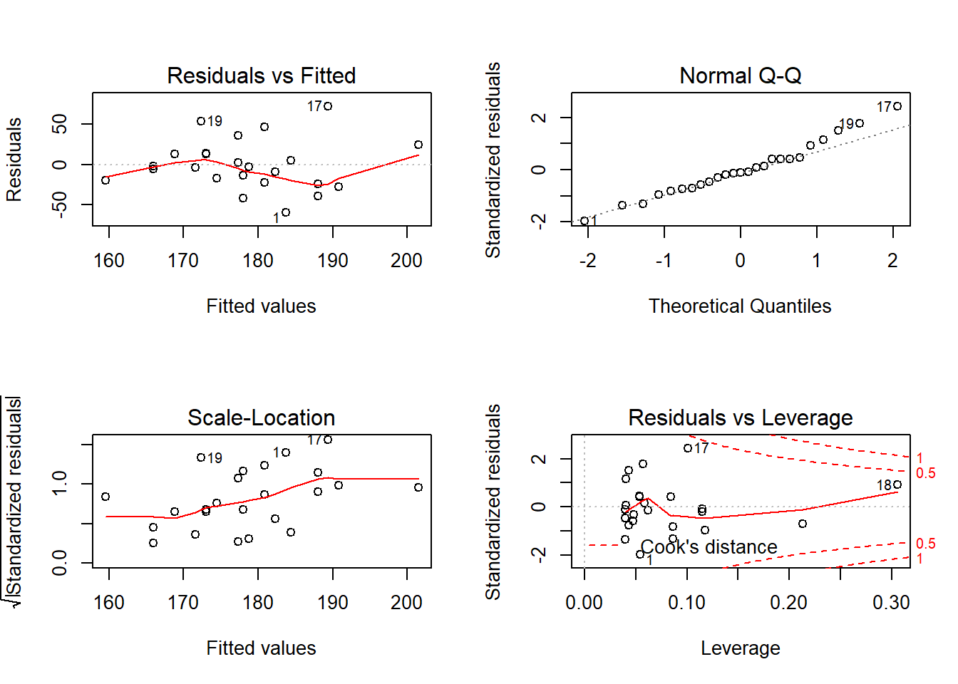

par(mfrow = c(1, 1))